Electromagnetic Fields and Waves: Notes, Solved Problems and Interactive Lab

Solve the source-free Helmholtz equation for the simplest field, $E = E_{x} (z) a_{x}$ , which depends on one coordinate only. Its divergence vanishes, and Eq. (5.6.17) reduces to the ordinary differential equation

⟹ \frac{d ^{2} E _{x}}{d z ^{2}} + k^{2} E_{x} = 0 E_{x} (z) = E_{0} e^{- j k z} + E_{0}^{'} e^{+ j k z} .

The first term is a wave towards $+ z$ , the second a wave towards $- z$ . Keep the first and write $k = β - j α$ :

E_{x} (z) E_{x} (z; t) = E_{0} e^{- j k z} = E_{0} e^{- α z} e^{- j β z}, = E_{0} e^{- α z} cos (ω t - β z) (5.6.19)

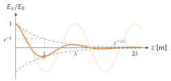
for a real $E_{0}$ . The phase constant $β$ fixes the phase, so $v_{p} = ω / β$ and $λ = 2 π / β$ , and the attenuation constant $α$ fixes the decay (Figure 5.6.9).

To find $β$ and $α$ , square $k = β - j α$ and compare with $k^{2} = ω^{2} μ ε (1 - j tan δ)$ from Eq. (5.6.16). The real and the imaginary parts give two real equations,

β^{2} - α^{2} = ω^{2} μ ε, 2 α β = ω^{2} μ ε tan δ .

Eliminate $α = ω^{2} μ ε tan δ /2 β$ from the first: $β^{4} - ω^{2} μ ε β^{2} - \frac{1}{4} (ω^{2} μ ε tan δ)^{2} = 0$ , a quadratic equation in $β^{2}$ whose positive root is $β^{2} = \frac{1}{2} ω^{2} μ ε [1 + 1 + tan^{2} δ]$ . Then $α^{2} = β^{2} - ω^{2} μ ε = \frac{1}{2} ω^{2} μ ε [1 + tan^{2} δ - 1]$ .

Phase and attenuation constants

β α = ω \frac{μ ε}{2} [1 + tan^{2} δ + 1]^{1/2} [rad/m], = ω \frac{μ ε}{2} [1 + tan^{2} δ - 1]^{1/2} [Np/m] . (5.6.20)

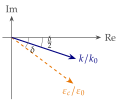
$k$ is the square root with $β > 0$ . Then $α \geq 0$ , the wave decays in the direction in which it travels, and $k$ lies in the fourth quadrant of the complex plane at the angle $ar g k = - δ /2$ .

In plain words

$β$ counts how fast the phase turns along the path, $α$ how fast the amplitude shrinks. In a lossless medium the wave keeps its amplitude for ever. With loss it fades as $e^{- α z}$ , and its power as $e^{- 2 α z}$ .

(a) A snapshot at t=0. — (a) A snapshot at $t = 0$ .

(b) \varepsilon_c and k. — (a) A snapshot at $t = 0$ .

Two other notations are common, and the book uses both where the sources do. Many texts write the wave as $e^{- γ z}$ with the propagation constant

γ = j k = α + j β, e^{- γ z} = e^{- j k z} = e^{- α z} e^{- j β z}, (5.6.21)

which puts the attenuation in the real part. The lecture works with $k = β - j α$ , the natural continuation of the real wave number $k_{0} = ω / c$ of a lossless medium. Both describe the same wave. The unit neper ( $Np$ ) is a natural logarithm of a ratio of field amplitudes: a field that falls by the factor $e^{- α l}$ over a length $l$ has lost $α l Np$ , which is $20 lo g_{10} e^{α l} = 8.686 α l dB$ .

Two limits are worth remembering. In a low-loss medium, $tan δ ≪ 1$ , the square roots of Eq. (5.6.20) expand to

β \approx ω μ ε, α \approx \frac{1}{2} β tan δ, (5.6.22)

and in a good conductor, $tan δ ≫ 1$ , both brackets tend to $tan δ$ , so that $α \approx β \approx ω μ σ /2 = π f μ σ$ . The consequences, the skin depth among them, are the subject of Section 6.2.

Quick check

Polyethylene has $ε_{r} = 2.25$ and $tan δ = 4 \times 1 0^{- 4}$ at $3 GHz$ . Find $β$ and the attenuation in $dB/m$ .

Low loss: $β \approx k_{0} ε_{r} = 62.83 \times 1.5 = 94.2 rad/m$ and $α \approx \frac{1}{2} \times 94.2 \times 4 \times 1 0^{- 4} = 0.0188 Np/m$ , that is $8.686 \times 0.0188 = 0.16 dB/m$ . The exact formulas of Eq. (5.6.20) give the same digits.

Common mistake · The wrong square root

$k^{2}$ has two square roots, $\pm (β - j α)$ . With the phasor $e^{- j k z}$ the wave that travels and decays towards $+ z$ needs $β > 0$ and $Im k < 0$ . Taking the other root, or writing $e^{+ j k z}$ with the same $k$ , describes a wave that grows as it travels, which a passive medium cannot produce. A quick test: $∣ e^{- j k z} ∣ = e^{(Im k) z}$ must fall as $z$ grows.

Application 5.6.2 · The microwave oven

Why water heats. Water molecules are permanent electric dipoles. An alternating $E$ makes them turn back and forth, and since they rub against their neighbours they lag behind the field. The polarisation, and with it $D$ , then lags $E$ , and $ε = ε^{'} - j ε^{''}$ has a loss part even in pure water, whose conductivity is negligible. The time-harmonic Poynting relation of Section 6.1 shows that a medium with $ε^{''}$ turns electromagnetic energy into heat at the average rate, per unit volume,

p_{a v} = \frac{1}{2} ω ε_{0} ε_{r}^{''} ∣ E ∣^{2} = \frac{1}{2} σ_{eff} ∣ E ∣^{2} [W/ m^{3}], (5.6.23)

the time average of the Joule heat $σ E^{2}$ with $σ \to σ_{eff}$ of Eq. (5.6.14). The frequency dependence of $ε_{r}$ is described well by the Debye model,

ε_{r} = ε_{\infty} + \frac{ε _{s} - ε _{\infty}}{1 + j ω τ}, ε_{s} = 78.4, ε_{\infty} = 5.2, τ = 8.27 ps (water at 25^{\circ} C), (5.6.24)

plotted in Figure 5.6.10. At low frequency the dipoles follow the field ( $ε_{r} \to ε_{s}$ ), at high frequency they cannot follow at all ( $ε_{r} \to ε_{\infty}$ ), and in between, around the relaxation frequency $1/2 π τ = 19 GHz$ , the loss $ε^{''}$ peaks. At the oven frequency of $2.45 GHz$

ε_{r} = 77.2 - j 9.2, tan δ = 0.12, σ_{eff} = 1.25 S/m . (5.6.25)

The complex permittivity of water at 25\,^\circ\mathrm C from the Debye model of Eq. (5.6.24). The real part falls from 78.4 to 5.2 as the dipoles stop following the field, and the loss \varepsilon''_r peaks at the relaxation frequency 1/2\pi\tau=19.2\,\mathrm{GHz}. The dots mark the oven frequency, where \varepsilon_r=77.2-j9.2. — **Figure 5.6.10.** The complex permittivity of water at $25^{\circ} C$ from the Debye model of Eq. (5.6.24). The real part falls from $78.4$ to $5.2$ as the dipoles stop following the field, and the loss $ε_{r}^{''}$ peaks at the relaxation frequency $1/2 π τ = 19.2 GHz$ . The dots mark the oven frequency, where $ε_{r} = 77.2 - j 9.2$ .

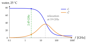
Why not heat at the peak, $19 GHz$ , where the loss is largest? Because the power of the wave falls as $e^{- 2 α z}$ (Worked example 5.6.1), and a large loss means a short reach. The depth at which the power has dropped to $1/ e$ , $1/2 α$ , is $13 cm$ at $915 MHz$ , $1.9 cm$ at $2.45 GHz$ and only $0.5 mm$ at $19 GHz$ . At the peak only the surface of the food would cook. The ISM frequency of $2.45 GHz$ is a compromise that reaches into the food and still heats it quickly. Industrial ovens use $915 MHz$ for thick loads.

Fields and power. A magnetron makes $700$ to $1000 W$ at $2.45 GHz$ ( $λ_{0} = 12.2 cm$ ). A short waveguide feeds a closed metal box in which the waves bounce off the walls and form standing waves (Figure 5.6.11). The hot spots repeat every $λ_{0} /2 = 6.1 cm$ , hence the turntable or a rotating mode stirrer that moves the food through them. The door is a metal mesh with holes of a few millimetres, far smaller than $λ_{0}$ : light passes, microwaves do not.

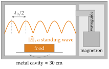
The microwave oven. The magnetron feeds the cavity through a short waveguide. The waves reflected by the metal walls form a standing wave whose maxima of |\vec E| repeat every \lambda_0/2=6.1\,\mathrm{cm}, and the turntable carries the food through them. — **Figure 5.6.11.** The microwave oven. The magnetron feeds the cavity through a short waveguide. The waves reflected by the metal walls form a standing wave whose maxima of $∣ E ∣$ repeat every $λ_{0} /2 = 6.1 cm$ , and the turntable carries the food through them.

How strong are the fields? For a plane wave in air the time-average power density is $∣ P_{a v} ∣ = E_{0}^{2} /2 η_{0}$ with $η_{0} = 120 π Ω$ (Section 6.1), and inside a lossy material the heat density is that of Eq. (5.6.23).

Power density and heat density

The power density of a plane wave of amplitude $E_{0}$ in air, and the heat density in a lossy medium where the field amplitude is $E_{0}$ , are

∣ P_{a v} ∣ p_{a v} = \frac{E _{0}^{2}}{2 η _{0}} [W/ m^{2}], = \frac{1}{2} σ_{eff} E_{0}^{2} [W/ m^{3}] . (5.6.26)

Table 5.6.4 puts in numbers. An oven's $800 W$ crossing a $30 \times 30 c m^{2}$ cross-section correspond to a plane wave of $2.6 kV/m$ . Absorbed by one litre of water, $800 W$ raise its temperature by $800/4180 = 0.19 K/s$ , about $11 K$ per minute, which inside the water needs only $E_{0} = 2 p_{a v} / σ_{eff} \approx 1.1 kV/m$ . Emission standards (US FDA, IEC 60335-2-25) allow at most $5 mW/c m^{2} = 50 W/ m^{2}$ at $5 cm$ from the oven surface.

Table 5.6.4. Power densities and the equivalent plane-wave amplitudes $E_{0} = 2 η_{0} ∣ P_{a v} ∣$ .

	$∣ P_{a v} ∣$	$E_{0}$
$800 W$ through $30 \times 30 c m^{2}$	$8.9 kW/ m^{2}$	$2.6 kV/m$
sunlight, top of the atmosphere	$1.36 kW/ m^{2}$	$1.0 kV/m$
oven leakage limit at $5 cm$	$50 W/ m^{2}$	$0.19 kV/m$

Quick check

At $2.45 GHz$ water has $σ_{eff} = 1.25 S/m$ . How large must the field amplitude in the water be to deposit $1 W/c m^{3}$ ?

$p_{a v} = 1 0^{6} W/ m^{3}$ , so $E_{0} = 2 p_{a v} / σ_{eff} = 2 \times 1 0^{6} /1.25 = 1.26 kV/m$ .

5.6.8 The complex wave number