5.5.4 The one-dimensional wave equation and d'Alembert's solution

Let the field depend on one coordinate only, besides time, and point along a fixed direction across it: $E = E_{x} (z, t) a_{x}$ . Then $\nabla \cdot E = \partial E_{x} / \partial x = 0$ automatically, and the Laplacian reduces to the second derivative in $z$ . The wave equation Eq. (5.5.14) becomes

\frac{\partial ^{2} E _{x}}{\partial z ^{2}} - \frac{1}{v ^{2}} \frac{\partial ^{2} E _{x}}{\partial t ^{2}} = 0. (5.5.16)

This equation can be solved in general, without any assumption about the shape of the field, by a change of variables due to J. le Rond d'Alembert (1747), who found it for the vibrating string.

1. New variables. Introduce

ξ = z - v t, η = z + v t, (5.5.17)

and regard $E_{x}$ as a function of $ξ$ and $η$ . Since $\partial ξ / \partial z = \partial η / \partial z = 1$ and $\partial ξ / \partial t = - v$ , $\partial η / \partial t = v$ , the chain rule gives

\frac{\partial}{\partial z} \frac{\partial}{\partial t} = \frac{\partial}{\partial ξ} + \frac{\partial}{\partial η}, = - v \frac{\partial}{\partial ξ} + v \frac{\partial}{\partial η} . (5.5.18)

2. Second derivatives. Applying each operator twice,

\frac{\partial ^{2}}{\partial z ^{2}} \frac{1}{v ^{2}} \frac{\partial ^{2}}{\partial t ^{2}} = \frac{\partial ^{2}}{\partial ξ ^{2}} + 2 \frac{\partial ^{2}}{\partial ξ \partial η} + \frac{\partial ^{2}}{\partial η ^{2}}, = \frac{\partial ^{2}}{\partial ξ ^{2}} - 2 \frac{\partial ^{2}}{\partial ξ \partial η} + \frac{\partial ^{2}}{\partial η ^{2}},

and the difference has a single term left:

\frac{\partial ^{2}}{\partial z ^{2}} - \frac{1}{v ^{2}} \frac{\partial ^{2}}{\partial t ^{2}} = 4 \frac{\partial ^{2}}{\partial ξ \partial η} ⟹ \frac{\partial ^{2} E _{x}}{\partial ξ \partial η} = 0. (5.5.19)

3. Integrate twice. $\partial (\partial E_{x} / \partial ξ) / \partial η = 0$ says that $\partial E_{x} / \partial ξ$ does not depend on $η$ : it is some function $F (ξ)$ of $ξ$ alone. Integrating once more in $ξ$ gives $E_{x} = \int F (ξ) d ξ + g (η) = f (ξ) + g (η)$ , where the "constant" of integration $g$ may depend on the other variable $η$ . Back in $z$ and $t$ :

d'Alembert's solution

Every solution of the one-dimensional wave equation Eq. (5.5.16) has the form

E_{x} (z, t) = f (z - v t) + g (z + v t) = F (t - \frac{z}{v}) + G (t + \frac{z}{v}), (5.5.20)

with $f$ and $g$ (equivalently $F$ and $G$ ) any twice differentiable functions, fixed by how the wave was launched. The term $f (z - v t)$ travels in the $+ z$ direction, $g (z + v t)$ in the $- z$ direction, both with the speed $v = 1/ μ ε$ and without change of shape.

In plain words

A wave is a shape that moves. Whatever shape the field has at $t = 0$ , the part $f$ slides to the right and the part $g$ to the left, rigidly, at the speed $v$ . The equation fixes the speed and nothing else.

The two forms in Eq. (5.5.20) are the same thing written twice. Any function of $z - v t$ is also a function of $t - z / v = - (z - v t) / v$ , namely $F (s) = f (- v s)$ , and likewise $G (s) = g (v s)$ . The first form is natural for snapshots in space at fixed $t$ , the second for signals in time at a fixed point $z$ : a receiver at $z$ sees $F (t - z / v)$ , the signal sent from $z = 0$ , delayed by $z / v$ .

Direct check. With $u = z - v t$ and $f^{'}$ , $f^{''}$ the derivatives with respect to the argument,

\frac{\partial f}{\partial z} \frac{\partial f}{\partial t} = f^{'} (u), = - v f^{'} (u), \frac{\partial ^{2} f}{\partial z ^{2}} \frac{\partial ^{2} f}{\partial t ^{2}} = f^{''} (u), = v^{2} f^{''} (u),

and $f^{''} - v^{- 2} v^{2} f^{''} = 0$ for every $f$ . The same holds for $g (z + v t)$ , with $+ v$ in place of $- v$ .

Following a point of the pulse. The peak of $f$ sits where its argument has the value $z_{0}$ it had at $t = 0$ , that is where $z - v t = z_{0}$ . So $z = z_{0} + v t$ and $d z / d t = v$ . Every other feature of the pulse, its front, its tail, a zero crossing, moves with the same speed, because each is a fixed value of the argument $z - v t$ . One number describes the whole motion (Figure 5.5.3). In the $(z, t)$ plane the lines $z - v t = const$ and $z + v t = const$ along which $f$ and $g$ keep their values are called the characteristics of the equation. They are the paths of the wave.

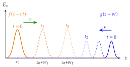
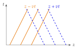
(a) Snapshots at t=0, t_1, t_2. — (a) Snapshots at $t = 0$ , $t_{1}$ , $t_{2}$ .

(b) Characteristics. — (a) Snapshots at $t = 0$ , $t_{1}$ , $t_{2}$ .

Press Play below and watch the two pulses, here in a dielectric with $ε_{r} = 4$ , pass through each other unchanged. Then change their shapes, or tap the space-time diagram to pick a time.

InteractiveLoading simulation…

What the mixed derivative equation says

Read Eq. (5.5.19), $\partial^{2} E_{x} / \partial ξ \partial η = 0$ , as a statement about information. The value carried by $f$ is fixed along each line $z - v t = const$ and the value carried by $g$ along each line $z + v t = const$ . A disturbance at one point and instant can influence another point only along these lines, so it needs the time $∣Δ z ∣/ v$ to arrive. This is the finite speed of electromagnetic signals in its most elementary form, and the retarded potentials of Section 5.5.10 are its three-dimensional version.

Common mistake · Reading the speed from one factor of a product

A field such as $sin (\frac{3}{2} x - 3 t) cos (\frac{1}{2} x - 9 t)$ contains two arguments that look like travelling waves with speeds $2$ and $18$ . Neither is the answer. A product of two functions is not in general a function of one combination $x \mp v t$ . Rewrite it as a sum first (Problem 5.5.1): it is two waves with the same speed $6$ moving in opposite directions. Likewise $sin 2 x cos 6 t$ is not a wave of speed $3$ moving anywhere but a standing wave, the sum of two equal waves moving in opposite directions.

Quick check

In which direction and with what speed does $u = e^{- (3 z + 6 t)^{2}}$ travel?

$3 z + 6 t = 3 (z + 2 t)$ , so $u$ is a function of $z + 2 t$ alone: a Gaussian pulse moving in the $- z$ direction with speed $2$ (in the units of $z$ and $t$ ). Check: $u_{z z} = 9 F^{''}$ and $u_{tt} = 36 F^{''}$ with $F$ the profile, so $u_{tt} / u_{z z} = 4 = v^{2}$ .