Electromagnetic Fields and Waves: Notes, Solved Problems and Interactive Lab

With walls of finite conductivity $σ_{c}$ the fields of the ideal guide drive surface currents $J_{S} = a_{n} \times H$ that flow in a skin of the wall and dissipate the power $P_{L}^{'} = \frac{1}{2} R_{s} \oint ∣ J_{S} ∣^{2} d l$ per unit length, with $R_{s} = π f μ_{0} / σ_{c}$ . As in Section 7.2, the power decays as $e^{- 2 α_{c} z}$ with $α_{c} = P_{L}^{'} / (2 P)$ . Carrying out the two integrals for the circular modes gives, with $s = 1 - (f_{c} / f)^{2}$ :

Conductor loss of a circular guide

α_{c}^{TM_{mn}} α_{c}^{TE_{mn}} = \frac{R _{s}}{a η s} [Np/m], = \frac{R _{s}}{a η s} [(\frac{f _{c}}{f})^{2} + \frac{m ^{2}}{x _{mn}^{'2} - m ^{2}}] . (7.4.23)

A lossy filling ( $ε = ε^{'} (1 - j tan δ)$ ) adds $α_{d} = k tan δ / (2 s)$ to every mode.

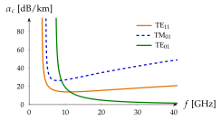
Figure 7.4.7 shows the three most important modes in a copper pipe of radius $2.5$ cm, whose cutoffs are $3.52$ (TE $_{11}$ ), $4.59$ (TM $_{01}$ ) and $7.32$ GHz (TE $_{01}$ ).

Every curve rises steeply at its cutoff: as $s \to 0$ the group velocity $v s$ goes to zero, the power crawls along while the wall currents stay.
TE $_{11}$ and TM $_{01}$ pass through a minimum and then grow as $f$ , the growth of $R_{s}$ . For TM modes the minimum lies at $f = 3 f_{c}$ (Exercise 7.4.2), for TE $_{11}$ near $3.15 f_{c}$ .
For TE $_{01}$ ( $m = 0$ ) the bracket in Eq. (7.4.23) is $(f_{c} / f)^{2}$ alone, and far above cutoff $α_{c} \propto R_{s} (f_{c} / f)^{2} \propto f^{- 3/2}$ . The loss falls without limit as the frequency rises. All the circularly symmetric TE $_{0 n}$ modes do this, and no other mode does.

Conductor attenuation of TE_{11}, TM_{01} and TE_{01} in an air-filled copper pipe (\sigma_c=5.8\times10^7 S/m) of radius a=2.5 cm, from Eq. (7.4.23). TE_{11} and TM_{01} have a minimum and then rise as \sqrt f. TE_{01} falls as f^{-3/2} far above its cutoff and is the lowest of the three above 11.4 GHz. — **Figure 7.4.7.** Conductor attenuation of TE $_{11}$ , TM $_{01}$ and TE $_{01}$ in an air-filled copper pipe ( $σ_{c} = 5.8 \times 1 0^{7}$ S/m) of radius $a = 2.5$ cm, from Eq. (7.4.23). TE $_{11}$ and TM $_{01}$ have a minimum and then rise as $f$ . TE $_{01}$ falls as $f^{- 3/2}$ far above its cutoff and is the lowest of the three above $11.4$ GHz.

The tool below shows the same copper pipe of radius $2.5 cm$ , with TE $_{01}$ at $15 GHz$ (Problem 7.4.2). Raise $f$ : TE $_{11}$ and TM $_{01}$ pass a minimum and rise, while TE $_{01}$ keeps falling.

InteractiveLoading simulation…

Why TE01 is special

At the wall TE $_{01}$ has only $H_{z}$ : $H_{ϕ} = 0$ because $m = 0$ , and $H_{ρ}$ is normal. The wall current $J_{S} = - a_{ρ} \times H_{z} a_{z} = H_{z} a_{ϕ}$ runs purely around the pipe. For a given power, the transverse field (which carries the power) grows relative to $H_{z}$ as the frequency rises, because $∣ H_{ρ} / H_{z} ∣ = τ / h$ grows with $τ$ . The wall current, and with it the loss, therefore shrinks relative to the power, faster than $R_{s}$ grows.

Quick check

Why does every curve in Figure 7.4.7 shoot up at its cutoff, although $R_{s}$ is perfectly finite there?

$α_{c} = P_{L}^{'} / (2 P)$ , and near cutoff the mode is almost a standing wave across the guide: $τ \to 0$ , the energy moves at $v_{g} = v s \to 0$ , and the power $P$ carried for a given field strength goes to zero. The wall currents, set by the field strength, do not. The factor $1/ s$ in Eq. (7.4.23) expresses exactly this.

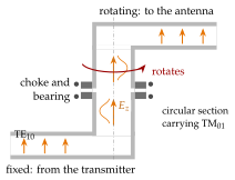
Application 7.4.1 · Rotary joints for radar antennas

A surveillance radar antenna turns continuously, its transmitter does not. The microwave path must cross a rotating interface with the same amplitude and phase at every angle of rotation. The TE $_{10}$ mode of a rectangular guide cannot do it, and neither can TE $_{11}$ : both have an electric field with a direction across the guide, which would turn with the antenna. TM $_{01}$ can, because its fields do not depend on $ϕ$ at all:

$E_{z} = C J_{0} (2.405 ρ / a) e^{- j τ z}$ , no $ϕ$ dependence

Figure 7.4.8 shows the principle.

The rectangular TE $_{10}$ mode of the fixed guide couples into TM $_{01}$ through a probe or a “doorknob” on the axis of the circular section. The field there is symmetric about the axis of rotation, and a second transition at the rotating end couples back into a rectangular guide.
The rotating gap is bridged by a quarter-wave choke: no sliding contact, no wear and little leakage. TM $_{01}$ has an axial wall current ( $J_{S} = - H_{ϕ} a_{z}$ ), which a plain gap would interrupt (Exercise 7.4.4).
TE $_{11}$ also propagates in the joint, since its cutoff is lower, and any asymmetry excites it. Mode filters (rings, absorbing vanes) suppress it.

A TM_{01} rotary joint, side view. The TE_{10} mode of the fixed rectangular guide is coupled into the circular section by a probe on its axis. The rotationally symmetric TM_{01} field, with E_z largest on the axis, crosses the rotating gap unchanged at any angle, and is coupled back into the rotating rectangular guide that leads to the antenna. A quarter-wave choke closes the gap for the axial wall current without metal contact. — **Figure 7.4.8.** A TM $_{01}$ rotary joint, side view. The TE $_{10}$ mode of the fixed rectangular guide is coupled into the circular section by a probe on its axis. The rotationally symmetric TM $_{01}$ field, with $E_{z}$ largest on the axis, crosses the rotating gap unchanged at any angle, and is coupled back into the rotating rectangular guide that leads to the antenna. A quarter-wave choke closes the gap for the axial wall current without metal contact.

Typical numbers. An X-band radar at $9.4$ GHz needs TM $_{01}$ to propagate and TE $_{21}$ , the next mode above it, to stay cut off: $2.405 < k a < 3.054$ , that is $12.2$ mm $< a < 15.5$ mm (Worked example 7.4.2). Joints with several channels nest a coaxial TEM channel, which is symmetric too, around or inside the TM $_{01}$ channel.

Application 7.4.2 · TE₀₁: the low-loss long-haul waveguide

In TE $_{01}$ the only magnetic field at the wall is $H_{z}$ , the wall current runs around the pipe, and the loss falls as $f^{- 3/2}$ far above cutoff (Section 7.4.9):

α_{c}^{TE_{01}} = \frac{R _{s}}{a η _{0}} \frac{( f _{c} / f ) ^{2}}{1 - ( f _{c} / f ) ^{2}} \propto f^{- 3/2}

For a copper pipe of $60$ mm diameter ( $a = 30$ mm, $f_{c} = 6.1$ GHz) the formula gives $0.94$ dB/km at $40$ GHz, $0.51$ dB/km at $60$ GHz and $0.20$ dB/km at $110$ GHz, while TE $_{11}$ in the same pipe loses $17$ to $28$ dB/km (Figure 7.4.9). In the 1960s and 1970s this promised a trunk line able to carry hundreds of thousands of telephone channels in millimetre-wave pipes buried in the ground.

The catch. At $60$ GHz the pipe is so large that about $700$ field patterns can propagate (the exact count is $709$ ). Every bend, dent or joint converts TE $_{01}$ into others, worst of all into TM $_{11}$ , which has the same cutoff and therefore the same phase velocity: nothing stops the conversion. The remedy was a lining of fine insulated helical wire. The helix carries the purely azimuthal current of TE $_{01}$ , but it is an open wall for every mode that needs an axial current, and these lose their power into the lossy jacket behind the helix (Exercise 7.4.4).

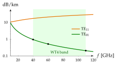
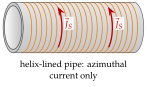
(b) The helix lining. — (a) Conductor loss in a 60 mm pipe.

History. Bell Laboratories (the WT4 system: $60$ mm pipe, $40$ to $110$ GHz, a $14$ km field trial in New Jersey in 1975) and the British Post Office ( $50$ mm pipe) built working trial lines. At the same time the optical fibre, proposed in 1966 and brought below $20$ dB/km in 1970, offered far more bandwidth in a far cheaper and more forgiving medium, and the pipes were never deployed. The same azimuthal-current physics lives on in the circular TE $_{01}$ -type cavity resonators of Section 7.8, prized for their high quality factor.

7.4.9 Attenuation in circular waveguides