7.5.6 Higher-order modes and the upper frequency limit

Besides the TEM wave the coaxial line supports TE and TM modes, built exactly as in the circular pipe of Section 7.4, with one difference: the field region is now the annulus $a < ρ < b$ . The axis is inside the inner conductor, the singularity of $Y_{m}$ at $ρ = 0$ is outside the region, and both solutions of Bessel's equation, Eq. (7.4.9) in Section 7.4, must be kept. For the TE $_{m 1}$ modes take

H_{z} = [J_{m} (h ρ) Y_{m}^{'} (ha) - Y_{m} (h ρ) J_{m}^{'} (ha)] \times cos m ϕ e^{- j τ z} . (7.5.15)

The combination is chosen so that $\partial H_{z} / \partial ρ = h [J_{m}^{'} (h ρ) Y_{m}^{'} (ha) - Y_{m}^{'} (h ρ) J_{m}^{'} (ha)] cos m ϕ$ vanishes at $ρ = a$ : the condition $E_{ϕ} = 0$ on the inner conductor is built in. On the outer conductor, $\partial H_{z} / \partial ρ = 0$ at $ρ = b$ gives the characteristic equation

J_{m}^{'} (ha) Y_{m}^{'} (hb) - J_{m}^{'} (hb) Y_{m}^{'} (ha) = 0, (7.5.16)

a transcendental equation for $h$ that is solved numerically. (For TM modes the same steps with $E_{z} = 0$ on both walls give $J_{m} (ha) Y_{m} (hb) - J_{m} (hb) Y_{m} (ha) = 0$ .) Its lowest root belongs to TE $_{11}$ , the first higher mode of the coaxial line, and lies very close to a simple estimate.

First higher mode of a coaxial line

h_{c} \approx \frac{2}{a + b}, λ_{c} \approx π (a + b), f_{c, TE_{11}} \approx \frac{v}{π ( a + b )} = \frac{c}{π ( a + b ) ε _{r}} . (7.5.17)

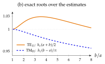
The coaxial line is single-mode (TEM only) below $f_{c, TE_{11}}$ . The exact root of Eq. (7.5.16) is at most $2.9 %$ above the estimate for $1 < b / a < 8$ .

In plain words

TE $_{11}$ is the TE $_{10}$ mode of a rectangular guide bent into a ring. It needs one full period of $cos ϕ$ around the mean circumference $π (a + b)$ , so it starts when the wavelength in the dielectric has shrunk to that circumference. The thinner the cable, the higher it can go.

(a) TE_{11} of a coax, \vec E lines. — (a) TE $_{11}$ of a coax, $E$ lines.

(b) Exact roots over the estimates. — (a) TE $_{11}$ of a coax, $E$ lines.

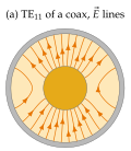
Above $f_{c, TE_{11}}$ a second mode, with its own phase and group velocities, can carry part of the power. Any discontinuity (a connector, a bend, a support bead) converts some TEM power into it, and the signal is distorted. Every cable and every connector therefore has an upper frequency limit set by Eq. (7.5.17), and the only way to raise it is to make the line smaller, which raises the loss ( $α_{c} \propto 1/ b$ at fixed $b / a$ ).

Quick check

The precision $7$ mm air line ( $2 a = 3.04$ mm, $2 b = 7.00$ mm) is rated to $18$ GHz. Why not higher?

$f_{c, TE_{11}} \approx 3 \times 1 0^{8} / (π \times 5.02 \times 1 0^{- 3}) = 19.0$ GHz (the exact root gives $19.4$ GHz). Above that TE $_{11}$ can propagate, so the rating stops just below. Exercise 7.5.2 shows that the support beads lower the limit further.

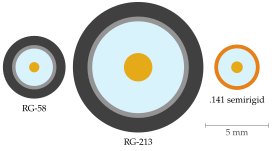
Application 7.5.1 · Coaxial cables and their frequency limits

Every laboratory bench is cabled with coaxial lines, and the formulas of this section explain their data sheets. Table 7.5.1 applies them to five standard cables, with smooth copper, polyethylene ( $ε_{r} = 2.25$ ) or PTFE ( $ε_{r} = 2.1$ ), both with $tan δ = 2 \times 1 0^{- 4}$ . Figure 7.5.6 draws three of them to scale.

Table 7.5.1. Standard coaxial cables computed with the formulas of this section: $Z_{0}$ from Eq. (7.5.8), the loss at $1$ GHz from Eq. (7.5.13) and the TE $_{11}$ cutoff from the estimate Eq. (7.5.17). SR: semirigid (solid copper tube). PE: polyethylene. $^{*}$ Stranded inner conductor, nominally $50 Ω$ . Measured losses of braided cables are higher.

cable, $2 a /2 b$ [mm]	$Z_{0}$ [ $Ω$ ]	$α$ at $1$ GHz [dB/m]	$f_{c, TE_{11}}$ [GHz]
RG-58 (PE), $0.81/2.95$	$51.7$	$0.37$	$34$
RG-213 (PE), $2.25/7.25$	$46. 8^{*}$	$0.17$	$13$
.141 SR (PTFE), $0.92/2.98$	$48.7$	$0.36$	$34$
.085 SR (PTFE), $0.51/1.68$	$49.4$	$0.62$	$60$
.047 SR (PTFE), $0.29/0.94$	$48.7$	$1.08$	$107$

Application 7.5.1. Three cables to scale: RG-58 and RG-213 with polyethylene (light blue), braided outer conductor (grey) and jacket (black), and the .141 semirigid cable with PTFE and a solid copper tube. The thick RG-213 loses less than half as much as RG-58 but stops at 13 GHz. — **Figure 7.5.6.** Application 7.5.1. Three cables to scale: RG-58 and RG-213 with polyethylene (light blue), braided outer conductor (grey) and jacket (black), and the .141 semirigid cable with PTFE and a solid copper tube. The thick RG-213 loses less than half as much as RG-58 but stops at $13$ GHz.

The key formula of the application is the frequency limit

$f_{m a x} \approx \frac{c}{π ( a + b ) ε _{r}}$ : thinner cable, higher limit, more loss

Precision connectors. Laboratory connectors are $50 Ω$ air lines with $b / a = 2.30$ , named after their outer diameter $2 b$ . Their TE $_{11}$ cutoffs, from the exact root of Eq. (7.5.16), set their ratings:

$2 b$ [mm]	$f_{c, TE_{11}}$ [GHz]	rated [GHz]
$7$	$19$	$18$
$3.5$	$39$	$26.5$
$2.92$	$47$	$40$
$2.4$	$57$	$50$
$1.85$	$73$	$67$
$1.0$	$136$	$110$

Each stops below its TE $_{11}$ cutoff, and the dielectric support beads lower the limit further: $40$ GHz measurements need $2.92$ mm parts, $110$ GHz needs $1$ mm parts. Worked example 7.5.1 compares two cables for a mast and shows why millimetre-wave radios are mounted at the antenna.