Electromagnetic Fields and Waves: Notes, Solved Problems and Interactive Lab

Without sources, Eq. (5.5.28) is

\nabla^{2} E - μ ε \frac{\partial ^{2} E}{\partial t ^{2}} - μ σ \frac{\partial E}{\partial t} = 0, (5.5.30)

and the same equation holds for $H$ . The new term contains the first time derivative. It acts like the friction on a vibrating string, or the resistor in an $R L C$ circuit: it takes energy out of the wave and turns it into the Joule heat $σ E^{2}$ per unit volume of Section 4.2.

Removing the friction term. The friction can be separated from the wave by the substitution

E = e^{- t / τ} u, τ = \frac{2 ε}{σ} . (5.5.31)

Problem 5.5.4 carries out the differentiation. The first time derivative of $u$ cancels exactly for this $τ$ , and $u$ obeys

\nabla^{2} u - \frac{1}{v ^{2}} \frac{\partial ^{2} u}{\partial t ^{2}} + α^{2} u = 0, α = \frac{σ}{2} \frac{μ}{ε} = \frac{1}{v τ} . (5.5.32)

For a signal of angular frequency $ω$ the term $v^{- 2} \partial^{2} u / \partial t^{2}$ has the size $(ω / v)^{2} u$ , and the extra term $α^{2} u$ is smaller than it by the factor $(α v / ω)^{2} = (1/ ω τ)^{2}$ . For a pulse much shorter than $τ$ ( $ω τ ≫ 1$ ) the extra term is negligible, $u$ obeys the lossless wave equation, and in one dimension $u = f (z - v t)$ . At the pulse itself $t = z / v$ , so $e^{- t / τ} = e^{- z / (v τ)} = e^{- α z}$ and

A pulse in a slightly conducting medium

For $ω τ ≫ 1$ , equivalently $σ ≪ ω ε$ , a pulse practically keeps its shape and its speed $v = 1/ μ ε$ , while its amplitude decays with the distance travelled:

E_{x} \approx e^{- α z} f (z - v t), α = \frac{σ}{2} \frac{μ}{ε} [Np/m] . (5.5.33)

In plain words

The main effect of a little conductivity is that the pulse fades: its amplitude falls by the factor $e$ over the distance $1/ α$ . The speed and the shape change too, but only very slightly. Both changes come from the term $α^{2} u$ neglected above. They are of second order in $σ / (ω ε)$ , while the attenuation is of first order. For a single frequency the phase velocity found in Section 6.2 is $v_{p} \approx v [1 - (σ / ω ε)^{2} /8]$ , a little below $v$ . Because this correction depends on the frequency, a pulse is also slightly distorted and leaves a weak wake behind it. For the moist sand of Problem 5.5.4, $σ / (ω ε) = 0.011$ and the speed is lower by only $1.6 \times 1 0^{- 5}$ of its value. Whenever $σ ≪ ω ε$ we ignore both effects.

The unit Np/m (neper per metre) marks $α$ as the rate of an exponential decay of the amplitude. One neper is $20 lo g_{10} e = 8.686 dB$ . Figure 5.5.6 shows the same pulse at four instants, with and without loss.

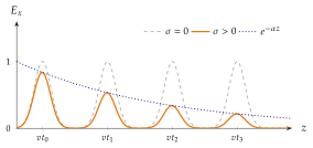
A short pulse at four instants t_0\lt t_1\lt t_2\lt t_3. In a lossless medium (dashed) it keeps its height. With a small conductivity it practically keeps its shape and its speed, but its amplitude follows the envelope e^{-\alpha z} (dotted). Here \alpha is exaggerated for visibility. — **Figure 5.5.6.** A short pulse at four instants $t_{0} < t_{1} < t_{2} < t_{3}$ . In a lossless medium (dashed) it keeps its height. With a small conductivity it practically keeps its shape and its speed, but its amplitude follows the envelope $e^{- α z}$ (dotted). Here $α$ is exaggerated for visibility.

The two limits. For a signal of angular frequency $ω$ the two time-derivative terms of Eq. (5.5.30) have the amplitudes $μ ε ω^{2}$ and $μ σ ω$ , in the ratio $σ / (ω ε) = 2/ (ω τ)$ . This is the loss tangent, Eq. (5.2.10) of Section 5.2 (Section 5.2.3), the ratio of the conduction current to the displacement current.

$σ ≪ ω ε$ , a good dielectric: a wave with a slowly decaying amplitude, as above. Example: moist sand at $200 MHz$ (Problem 5.5.4).
$σ ≫ ω ε$ , a good conductor: the second time derivative is negligible and Eq. (5.5.30) becomes $\nabla^{2} E = μ σ \partial E / \partial t$ , a diffusion equation, the equation of heat conduction. The field soaks into the conductor instead of travelling through it, and it is confined to a thin layer near the surface: the skin effect of Section 6.2.

Exercise 5.5.3 places three real materials on this scale. For a single frequency the decay constant can be found exactly (Home exercise 5.5.1): a field $E_{0} e^{- α z} cos (ω t - β z)$ solves Eq. (5.5.30) if $β^{2} - α^{2} = ω^{2} μ ε$ and $2 α β = ω μ σ$ , and for $σ ≪ ω ε$ this $α$ tends to Eq. (5.5.33). In the phasor language of Section 5.6 the same field is $E_{0} e^{- γ z}$ with the propagation constant $γ = α + j β$ . Some books, and the lecture slides, write it as $e^{- j k z}$ with the complex wave number $k = β - j α$ , which is the same thing since $j k = α + j β = γ$ .

Quick check

Dry sand has $ε_{r} = 4$ and $σ = 1 0^{- 4} S/m$ . Is it a good dielectric at $100 MHz$ , and over what distance does a radar pulse lose a factor $e$ of its amplitude?

$σ / (ω ε) = 1 0^{- 4} / (2 π \times 1 0^{8} \times 4 \times 8.842 \times 1 0^{- 12}) = 0.0045 ≪ 1$ : a good dielectric. $α = \frac{σ}{2} μ_{0} / (4 ε_{0}) = 5 \times 1 0^{- 5} \times 60 π = 0.0094 Np/m$ , so $1/ α = 106 m$ . Dry sand is almost transparent to radar, wet soil is not (Problem 5.5.4).

5.5.7 The loss term: a wave in a conducting medium