Electromagnetic Fields and Waves: Notes, Solved Problems and Interactive Lab

About the further exercises of Section 6.4

Ten further exercises in the spirit of Problems 6.4.1–6.4.6 and the home exercises, in two groups each graded from easy to harder: Exercises 6.4.1–6.4.5 on the coefficients, the critical angle and the Brewster angle, Exercises 6.4.6–6.4.10 on applications in radio, fibre optics, microscopy, radomes and metal walls. They use only the equations listed at the head of this subsection and, where stated, the normal-incidence results of Section 6.3.

Exercise 6.4.10

A copper wall at oblique incidence

A $10 GHz$ plane wave in air falls at the angle $θ_{i}$ on a flat copper surface ( $σ = 5.8 \times 1 0^{7} S/m$ ). (a) Find $R_{s}$ and $δ$ , and show that $θ_{t} \approx 0$ for every $θ_{i}$ . (b) Taking $cos θ_{t} = 1$ , show that the absorbed fractions are $A_{⊥} \approx 4 R_{s} cos θ_{i} / η_{0}$ and $A_{∥} \approx 4 R_{s} / (η_{0} cos θ_{i})$ as long as $η_{0} cos θ_{i} ≫ ∣ η_{2} ∣$ , and evaluate them at $0^{\circ}$ , $6 0^{\circ}$ and $8 0^{\circ}$ . (c) Find the exact $A_{∥} (θ_{i})$ (still with $cos θ_{t} = 1$ ), its maximum and the angle where it occurs. (d) Check (b) by the power-loss method: the power absorbed per unit area of a good conductor is $\frac{1}{2} R_{s} ∣ H_{t a n} ∣^{2}$ , with $H_{t a n}$ taken from the perfect-conductor solution.

Try it yourself first.

Strategy

In a good conductor $∣ γ_{2} ∣ ≫ β_{1}$ , so Snell's law forces $sin θ_{t} \approx 0$ : the wave enters the metal along the normal at every angle of incidence. With $cos θ_{t} = 1$ the Fresnel formulas contain $η_{2} cos θ_{i}$ (S) and $η_{0} cos θ_{i}$ (P), and $1 - ∣Γ ∣^{2} = 4 Re {a} b /∣ a + b ∣^{2}$ for $Γ = (a - b) / (a + b)$ with real $b$ . For a good conductor $η_{2} \approx (1 + j) R_{s}$ with $R_{s} = π f μ / σ$ (Section 6.2).

$R_{s} = π f μ_{0} / σ = 0.0261 Ω$ , $η_{2} = 0.0261 (1 + j) Ω$ , $δ = 1/ π f μ_{0} σ = 0.661 μ m$ . Since $β_{1} = 209 rad/m$ and $∣ γ_{2} ∣ = 2 / δ = 2.14 \times 1 0^{6} m^{- 1}$ , $∣ sin θ_{t} ∣ \leq β_{1} /∣ γ_{2} ∣ = 9.8 \times 1 0^{- 5}$ : $θ_{t} < 0.00 6^{\circ}$ .

S: $Γ_{⊥} = \frac{η _{2} cos θ _{i} - η _{0}}{η _{2} cos θ _{i} + η _{0}}$ , so $A_{⊥} = \frac{4 R _{s} cos θ _{i} η _{0}}{∣ η _{2} cos θ _{i} + η _{0} ∣ ^{2}} \approx \frac{4 R _{s} cos θ _{i}}{η _{0}}$ . P: $Γ_{∥} = \frac{η _{2} - η _{0} cos θ _{i}}{η _{2} + η _{0} cos θ _{i}}$ , so $A_{∥} = \frac{4 R _{s} η _{0} cos θ _{i}}{∣ η _{2} + η _{0} cos θ _{i} ∣ ^{2}} \approx \frac{4 R _{s}}{η _{0} cos θ _{i}}$ . With $4 R_{s} / η_{0} = 2.77 \times 1 0^{- 4}$ :

0^{\circ} 6 0^{\circ} 8 0^{\circ} : A_{⊥} = A_{∥} = 2.77 \times 1 0^{- 4}, : 1.38 \times 1 0^{- 4}, 5.54 \times 1 0^{- 4}, : 4.8 \times 1 0^{- 5}, 1.59 \times 1 0^{- 3} .

With $u = η_{0} cos θ_{i}$ , $∣ η_{2} + u ∣^{2} = (R_{s} + u)^{2} + R_{s}^{2}$ and

A_{∥} \frac{d A _{∥}}{d u} = \frac{4 R _{s} u}{( R _{s} + u ) ^{2} + R _{s}^{2}}, = 0 \Rightarrow u^{2} = 2 R_{s}^{2}, u = 2 R_{s},

A_{∥, m a x} at cos θ_{i} θ_{i} = \frac{4 2}{( 1 + 2 ) ^{2} + 1} = 2 (2 - 1) = 0.828 = \frac{2 R _{s}}{η _{0}} = 9.8 \times 1 0^{- 5}, = 89.99 4^{\circ} .

At a perfect conductor the tangential $H$ is $2 H_{0} cos θ_{i}$ for S (Problem 6.4.4) and $2 H_{0}$ for P (Home exercise 6.4.4), while the incident wave brings $\frac{1}{2} η_{0} H_{0}^{2} cos θ_{i}$ per unit area of the wall:

A_{⊥} A_{∥} = \frac{\frac{1}{2} R _{s} 4 H _{0}^{2} cos ^{2} θ _{i}}{\frac{1}{2} η _{0} H _{0}^{2} cos θ _{i}} = \frac{4 R _{s} cos θ _{i}}{η _{0}}, = \frac{\frac{1}{2} R _{s} 4 H _{0}^{2}}{\frac{1}{2} η _{0} H _{0}^{2} cos θ _{i}} = \frac{4 R _{s}}{η _{0} cos θ _{i}},

the same as in (b).

Answer

R_{s} = 0.0261 Ω, δ = 0.661 μ m, A_{⊥} \approx \frac{4 R _{s} cos θ _{i}}{η _{0}}, A_{∥} \approx \frac{4 R _{s}}{η _{0} cos θ _{i}}, A_{∥, m a x} = 2 (2 - 1) = 82.8 % at θ_{i} = 89.99 4^{\circ}

Check

The full Fresnel formulas with the complex $cos θ_{t}$ give $A_{∥} = 1.593 \times 1 0^{- 3}$ at $8 0^{\circ}$ (approximation $1.594 \times 1 0^{- 3}$ ) and the same maximum $0.8284$ . The maximum does not depend on $R_{s}$ : every good conductor absorbs $82.8 %$ of a P wave at the angle where $η_{0} cos θ_{i} = 2 R_{s}$ .

Exercise 6.4.10. The fractions of the incident power absorbed by copper at 10\,\mathrm{GHz}, against the grazing angle 90^\circ-\theta_i on logarithmic scales. Far from grazing A_\parallel grows as 1/\cos\theta_i and A_\perp falls as \cos\theta_i. The P absorption peaks at 82.8\,\% only 0.0056^\circ from grazing. — **Figure 6.4.24.** Exercise 6.4.10. The fractions of the incident power absorbed by copper at $10 GHz$ , against the grazing angle $9 0^{\circ} - θ_{i}$ on logarithmic scales. Far from grazing $A_{∥}$ grows as $1/ cos θ_{i}$ and $A_{⊥}$ falls as $cos θ_{i}$ . The P absorption peaks at $82.8 %$ only $0.005 6^{\circ}$ from grazing.

Remark

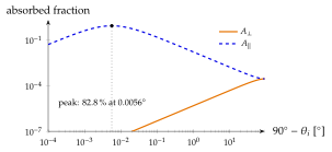
The P wave has a normal $E$ and a tangential $H$ that stays at $2 H_{0}$ even at grazing incidence, while the power it brings per unit area of wall vanishes as $cos θ_{i}$ : hence $A_{∥}$ grows towards grazing. For copper at $10 GHz$ the peak lies only $0.00 6^{\circ}$ from grazing. At optical frequencies, where $∣ η_{2} ∣$ is much larger (Exercise 6.3.6), it moves to angles of $7 0^{\circ}$ to $8 0^{\circ}$ and is used to characterise metal surfaces. The power-loss method of (d) is exactly how the wall losses of waveguides are computed in Chapter 7.

cf. Problem 6.4.4

Exercise 6.4.10: A copper wall at oblique incidence