Electromagnetic Fields and Waves: Notes, Solved Problems and Interactive Lab

The eigenvalue equations involve $h$ , $α$ and $d$ only through the products $h d /2$ and $α d /2$ . Multiply Eq. (7.6.8) by $(d /2)^{2}$ and define the dimensionless quantities

u = \frac{h d}{2}, w = \frac{α d}{2} . (7.6.18)

The relation $h^{2} + α^{2} = k_{0}^{2} (n_{1}^{2} - n_{2}^{2})$ becomes $u^{2} + w^{2} = V^{2}$ , a circle in the $u$ – $w$ plane whose radius depends only on the guide and the frequency:

Normalised frequency and the normalised eigenvalue equations

V NA = \frac{k _{0} d}{2} NA = \frac{π d}{λ _{0}} n_{1}^{2} - n_{2}^{2}, = n_{1}^{2} - n_{2}^{2}, (7.6.19)

u^{2} + w^{2} = V^{2}, TE_{m} : w = u tan (u - \frac{mπ}{2}), TM_{m} : w = \frac{n _{2}^{2}}{n _{1}^{2}} u tan (u - \frac{mπ}{2}) . (7.6.20)

For even $m$ the right-hand side is $u tan u$ , for odd $m$ it is $- u cot u$ (times $n_{2}^{2} / n_{1}^{2}$ for TM).

In plain words

Every symmetric slab, of any size, material and frequency, is described by one number, $V$ . Two slabs with the same $V$ have the same modes in normalised form, and only the conversion back to $h$ , $α$ and $τ$ differs.

The quantity $NA$ is the numerical aperture. Its name comes from the optical fibre, where it fixes the cone of light a fibre accepts (Section 7.6.10). The equations Eq. (7.6.20) have no closed-form solution, but they are easy to solve in two ways.

Graphically

Plot the branches $w = u tan u$ (on $0 \leq u < π /2$ , $π \leq u < 3 π /2$ , …) and $w = - u cot u$ (on $π /2 \leq u < π$ , …) in the first quadrant of the $u$ – $w$ plane, together with the quarter circle of radius $V$ . Each intersection is a mode, the branch tells which one, and the coordinates of the intersection are its $(u, w)$ (Figure 7.6.4). A small circle ( $V = 1.2$ ) cuts only the first branch: only TE $_{0}$ is guided. A larger one ( $V = 3.5$ ) cuts three branches: TE $_{0}$ , TE $_{1}$ and TE $_{2}$ . The TM branches lie below the TE branches (they are reduced by $n_{2}^{2} / n_{1}^{2} < 1$ ), so each TM root lies slightly to the right of its TE partner.

Numerically

On the branch of mode $m$ , $mπ /2 \leq u < (m + 1) π /2$ , the function $f (u) = u tan (u - mπ /2) - V^{2} - u^{2}$ increases monotonically from a negative value to $+ \infty$ (or to a positive value at $u = V$ ), so it has exactly one zero there if $V > mπ /2$ . Bisection on that interval, or Newton's method, finds it to any accuracy in a few steps.

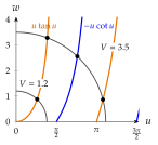
Graphical solution of the TE eigenvalue equations Eq. (7.6.20). Orange: the even branches w=u\tan u, blue: the odd branches w=-u\cot u. The quarter circles u^2+w^2=V^2 cut them at the modes (dots). For V=1.2 only TE_0 exists, at (u,w)=(0.819,0.877). For V=3.5 there are three modes, (1.216,3.282), (2.390,2.557) and (3.391,0.865): TE_0, TE_1 and TE_2. — **Figure 7.6.4.** Graphical solution of the TE eigenvalue equations Eq. (7.6.20). Orange: the even branches $w = u tan u$ , blue: the odd branches $w = - u cot u$ . The quarter circles $u^{2} + w^{2} = V^{2}$ cut them at the modes (dots). For $V = 1.2$ only TE $_{0}$ exists, at $(u, w) = (0.819, 0.877)$ . For $V = 3.5$ there are three modes, $(1.216, 3.282)$ , $(2.390, 2.557)$ and $(3.391, 0.865)$ : TE $_{0}$ , TE $_{1}$ and TE $_{2}$ .

The tool below starts with the $ε_{r} = 5$ sheet of Problem 7.6.1 ( $d = 2 cm$ , $10 GHz$ ). Raise $f$ and watch the circle reach the next branch: a new mode is born at $n_{eff} = n_{2}$ .

InteractiveLoading simulation…

Recipe · Finding the modes of a dielectric slab

Compute $NA = n_{1}^{2} - n_{2}^{2}$ and $V = (π d / λ_{0}) NA$ .
The TE $_{m}$ and TM $_{m}$ modes with $mπ /2 < V$ are guided: $m = 0, 1, \dots, ⌊ 2 V / π ⌋$ .
For each of them solve $w = u tan (u - mπ /2)$ (times $n_{2}^{2} / n_{1}^{2}$ for TM), $w = V^{2} - u^{2}$ , on $mπ /2 < u < min {(m + 1) π /2, V}$ , by bisection.
Convert back: $h = 2 u / d$ , $α = 2 w / d$ , $τ = k_{0}^{2} n_{1}^{2} - h^{2} = k_{0}^{2} n_{2}^{2} + α^{2}$ , $n_{eff} = τ / k_{0}$ , $λ_{g} = 2 π / τ$ .
Check: $n_{2} < n_{eff} < n_{1}$ , and $u^{2} + w^{2} = V^{2}$ .

Quick check

Verify the root of Figure 7.6.4 for $V = 1.2$ .

$u tan u = 0.819 \times tan 0.819 = 0.819 \times 1.071 = 0.877 = w$ (the angle in radians), and $u^{2} + w^{2} = 0.671 + 0.769 = 1.440 = 1. 2^{2}$ . Both equations are satisfied.

7.6.5 Normalised form and the graphical solution

Graphically

Numerically