Section 7.3 · Topic 6 of 11
7.3.6 The dominant TE₁₀ mode
The fields
Put , and into the TE formulas (7.3.23) and (7.3.21). Nothing depends on , so every vanishes, and
The constant is an amplitude of , but in practice one specifies the electric field. Call the peak electric field , that is . Then , and with :
all other components zero, with
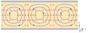
In the TE mode the electric field points straight from the bottom wall to the top wall, is strongest in the middle of the guide and vanishes at the narrow walls. The magnetic field forms loops lying flat in the guide, with a transverse part in step with and a longitudinal part a quarter period out of step with it.
TE is the working mode of practically every rectangular guide, for three reasons.
- It has the lowest cutoff of all modes, so for a given frequency it needs the smallest guide.
- It has an octave of single-mode band when , from to .
- Its has one fixed direction () and depends neither on nor on : the height is free to be chosen for power and loss, as the following subsections show.
The real fields
With real, the instantaneous fields are the real parts of the phasors (7.3.29) times . Since ,
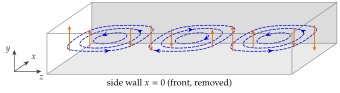
Figure 7.3.5 shows them at , for and over guide wavelengths. The lines of lie in planes const and are closed. They are the contours of , as one checks from Eq. (7.3.31): and of that function. The loops sit between the maxima of , a quarter of away from them, and the whole pattern slides along at the phase velocity.
TE₁₀ as two plane waves
Split the sine of Eq. (7.3.29) into exponentials, :
Each term is a uniform plane wave, with the wave vectors . Their length is by Eq. (7.3.2), the wavenumber of the filling, so these are ordinary plane waves of the medium (Chapter 6). They bounce between the narrow walls and at the angle to the axis given by
TE is an ordinary plane wave zig-zagging between the narrow walls. The closer the frequency is to cutoff, the steeper the zig-zag, the longer the guide wavelength and the slower the energy moves down the guide.
Their () is parallel to the narrow walls, and at each reflection from a perfect conductor the reflection coefficient is (Section 6.4): incident and reflected fields cancel on the wall, so at and . Figure 7.3.6 draws the rays.
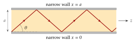
At cutoff and : the waves bounce straight across the guide without progress along it, and . Above cutoff the wavefronts meet the axis obliquely, so the crests along are spaced apart and move at , while the energy, which travels along the rays at , advances along at . This is exactly the picture of the parallel-plate guide of Section 7.2, with the width in place of the plate spacing. The broad walls meet a normal and play no role in the bouncing: this is why is absent from .
At which angle do the plane waves of TE travel at , and how long is the guide wavelength compared with ?
, so and . The phase velocity is and the group velocity .
Surface currents and charges on the walls
On a perfect conductor the tangential is carried by a surface current and the normal ends on a surface charge (Sections 4.2.3 and 3.4.6). With the unit normal pointing into the guide,
For TE, with and :
-
Top wall , : and .
-
Bottom wall , : the negative of both, , .
-
Side walls () and (): only is tangential, and on both walls
since and with .
On the broad walls is largest on the centre line and is largest at the edges. The current therefore flows along near the middle of the broad walls, crosswise near their edges, and vertically on the narrow walls (Figure 7.3.7). It does not close on the walls: where it converges, charge accumulates, and the circuit closes through the displacement current that crosses the guide from wall to wall (Exercise 7.3.4 verifies the continuity equation of Section 5.4).
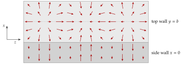
On the centre line of the broad wall is purely longitudinal. A narrow slot cut along it interrupts no current and hardly disturbs the guide: this is the slotted measuring line. A slot that cuts current lines, off the centre line or transverse to it, forces the current across a gap. The interrupted current continues as a displacement current across the slot, which then radiates like a small antenna: the slot antennas of Application 7.3.2.
The tool below shows the walls of the TE guide of Problem 7.3.2 (, , ). Press Play: the current along the centre line is purely longitudinal while the whole pattern slides at .
Power flow
The time-average Poynting vector is . With and ,
The longitudinal component is
while , because is imaginary: the crosswise flow is purely reactive, energy sloshing between the narrow walls. Integrating over the cross-section, , , with the mean value of over the width:
The power is the peak power density times half the cross-section. It grows with the area and vanishes at cutoff, where .
The power limit
The peak field must stay below the breakdown field of the filling, about for dry air at atmospheric pressure (Section 3.4.4). For WR-90 at (, , ) this gives
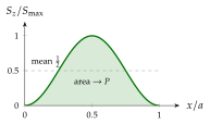
For a single mode with (TM) or (TE), the transverse fields are proportional to , and reduces to
Green's first identity and give , because on the wall either (TM) or (TE). With (and for a cosine with index zero):
For TE, with and , the TE formula gives back Eq. (7.3.37). Below cutoff is imaginary and : an evanescent mode carries no power.
A TE guide carries with the peak field . What happens to if (a) is doubled, (b) is halved at the same , (c) the frequency moves closer to cutoff at the same ?
(a) : four times the power. (b) : half the power. (c) grows, so falls, and at cutoff it is zero. A guide used close to cutoff has a poor power rating.
Attenuation due to the walls
Real walls have a finite conductivity , and the current (7.3.34) flows in a skin of depth (Section 6.2). Its loss is described by the surface resistance
For good conductors the fields hardly differ from those of the lossless guide, so the loss can be computed with the lossless currents (the perturbation method of Section 7.2). The power lost per unit length of guide is
taken round the perimeter of the cross-section. With the TE currents of the previous subsection:
- each broad wall contributes , since the mean of and of over the width is ,
- each narrow wall contributes .
Adding two of each (broad walls, then narrow walls):
The bracket simplifies. Since and ,
so . The power along the guide decays as , so and . Dividing by twice Eq. (7.3.37):
The wall currents heat the walls. The loss grows near cutoff, where the waves bounce almost straight across and is large, and it falls as , because a taller guide spreads the same current over more wall.
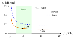
is the attenuation constant of the field, . The power falls twice as fast, . In decibels the two agree, for either, but a fraction of power computed as is wrong. Over of WR-137 at (Problem 7.3.4) the correct becomes a wrong .