3.4.6 Electrostatic boundary conditions

Real problems involve several media: a cable has a metal conductor, a plastic insulation and a metal screen, a capacitor has plates and a dielectric, and a raindrop is water in air. At the surface where two media meet, $\epsilon$ jumps, and the fields themselves may jump. The differential equations (3.4.5) cannot be applied across such a surface, because the derivatives do not exist there. The integral forms, however, remain valid for any contour and any surface, and from them we shall now derive how the fields on the two sides of an interface are related. The plan has two steps: a small loop straddling the interface will tell us about the tangential components, and a small pillbox about the normal components.

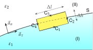
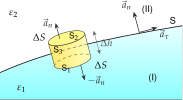
Let the surface S separate region I, of permittivity ${\epsilon }_1$, from region II, of permittivity ${\epsilon }_2$ (Figure 3.4.11). At a point of S let $a_n$ be the unit normal pointing from region I into region II and $a_{\tau }$ a unit vector tangent to S. Near the surface we decompose the fields into tangential and normal components,

and we label the values just below S (in region I) with the subscript 1 and those just above S (in region II) with the subscript 2.

The tangential component of E

Apply the first fundamental equation, ${\oint }_{C}E\cdot dl=0$, to the small rectangular loop C of Figure 3.4.11(a). Its sides C${}_1$ and C${}_3$, of length $\Delta l$, run parallel to S, one on each side, while the short sides C${}_2$ and C${}_4$, of length $\Delta h$, cross S. The loop integral is the sum of four line integrals,

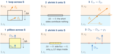
Now let the loop shrink onto the surface, $\Delta h\to 0$, keeping $\Delta l$ fixed but small enough for the field to be practically constant along each side (Figure 3.4.12, top row).

• On C${}_1$, which lies in region I and is traversed in the direction $+a_{\tau }$, $dl=a_{\tau }dl$, and the integral tends to $E_1\cdot a_{\tau }\Delta l=E_{1\tau }\Delta l$.
• On C${}_2$ and C${}_4$ the field is finite while the path length $\Delta h$ tends to zero, so ${\int }_{C_2+C_4}E\cdot dl\to 0$.
• On C${}_3$, which lies in region II and is traversed in the direction $-a_{\tau }$, the integral tends to $-E_{2\tau }\Delta l$.

Therefore

and since $\Delta l\ne 0$,

The tangential component of $E$ is continuous across any interface. Because the loop can be oriented along any tangential direction, the whole tangential part of $E$ is continuous, which can be written compactly as $a_n\times E_1=a_n\times E_2$. The derivation never used the nature of the media, nor the presence or absence of surface charge: a sheet of charge on S affects only the normal component of the field, as we shall now see.

The normal component of D

Apply the second fundamental equation, ${\oint }_{S}D\cdot dS={\int }_v{\rho }_{v}dv$, to the small pillbox of Figure 3.4.11(b). Its two faces, of area $\Delta S$, are parallel to S, one on each side, and its side S${}_3$ has the height $\Delta h$. Again let $\Delta h\to 0$ (Figure 3.4.12, bottom row).

• On the face S${}_1$, in region I, the outward normal is $-a_n$, so $dS=-a_{n}dS$ and the flux tends to $D_1\cdot (-a_n)\Delta S=-D_{1n}\Delta S$.
• On the face S${}_2$, in region II, the outward normal is $+a_n$ and the flux tends to $D_{2n}\Delta S$.
• The area of the side S${}_3$ is proportional to $\Delta h$, so its flux tends to zero.

On the right-hand side, a finite volume charge density ${\rho }_v$ contributes ${\rho }_v\Delta S\Delta h\to 0$. If, however, the interface carries a surface charge of density ${\rho }_S$ [C/m${}^2$], the pillbox encloses the charge ${\rho }_S\Delta S$ however thin it is:

Equating the two sides, $D_{2n}\Delta S-D_{1n}\Delta S={\rho }_S\Delta S$, and therefore

In vector form, $a_n\cdot (D_2-D_1)={\rho }_S$ with $a_n$ pointing from region I into region II. The normal component of $D$ jumps by the free surface charge density. If the interface carries no free charge, $D_n$ is continuous. Here ${\rho }_S$ is the free charge only: the bound charges on the two faces of the interface are already accounted for through ${\epsilon }_1$ and ${\epsilon }_2$. (The normal component of ${\epsilon }_{0}E$, by contrast, jumps by the total, free plus bound, surface charge. See Exercise 3.4.1.)

Summary of the boundary conditions

Using $D=\epsilon E$ and $E=-\nabla V$, each condition can be written in three equivalent forms. For the potential, the first condition means that $V$ is continuous: the potential difference between two points on opposite sides of S, a distance $\Delta h$ apart, is $-\int E\cdot dl\to 0$ because $E$ is finite. For the second condition we use $E_n=-\partial V/\partial n$, the derivative along $a_n$: $D_{2n}-D_{1n}=-{\epsilon }_2\partial V_2/\partial n+{\epsilon }_1\partial V_1/\partial n$.

These conditions, together with Poisson's or Laplace's equation in each region, determine the field completely. In practice we solve the differential equation in each region separately and then fix the integration constants with the boundary conditions, exactly as in Home exercise 3.4.3.

Refraction of E at a charge-free interface

What happens to a field line when it crosses an interface without free charge? Let $\theta$ denote the angle between $E$ and the normal $a_n$, so that $\tan \theta =E_{\tau }/E_n$. With ${\rho }_S=0$ the two boundary conditions read

Dividing the first by the second eliminates the field strength:

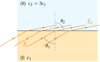
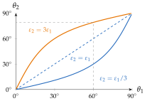
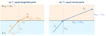
For the lines drawn in Figure 3.4.14, ${\theta }_1=60^{\circ }$ and ${\epsilon }_2=3{\epsilon }_1$ give $\tan {\theta }_2=3\tan 60^{\circ }=5.20$, i.e. ${\theta }_2=79.1^{\circ }$. Let us read the picture carefully. Since there is no surface charge, the lines drawn may be taken as lines of $D$, which has the same direction as $E$ in each medium. They are continuous: $D_n$ is the same on both sides, so no line of $D$ starts or ends on S. They bend away from the normal in the medium of higher permittivity, and there they crowd together. Indeed $|D_2|>|D_1|$, because $D_n$ is equal on both sides while $D_{\tau }=\epsilon E_{\tau }$ is three times larger in region II. Yet $|E_2|<|E_1|$, because $E_{\tau }$ is equal while $E_n$ is divided by ${\epsilon }_2/{\epsilon }_1=3$ (Figure 3.4.13).

The limiting cases are instructive. A line that meets the interface normally (${\theta }_1=0$) or tangentially (${\theta }_1=90^{\circ }$) does not bend at all. If region II has a much higher permittivity than region I, ${\theta }_2\to 90^{\circ }$: inside a high-permittivity body the field lines run almost parallel to its surface. Conversely, lines leaving a high-permittivity medium (water, ${\epsilon }_r\approx 80$, say) into air emerge almost perpendicular to the surface, whatever their direction inside. This is the same behaviour that we shall find, in the extreme, at the surface of a conductor (Section 3.4.7).

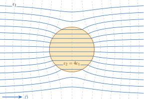
Figure 3.4.15 shows all of this at once for a dielectric cylinder in a uniform field $E_0$. Inside the cylinder the field is uniform and weaker, $E=2{\epsilon }_1{E}_0/({\epsilon }_1+{\epsilon }_2)=0.4E_0$ for ${\epsilon }_2=4{\epsilon }_1$, while the flux density $D={\epsilon }_{2}E=1.6{\epsilon }_1{E}_0$ is stronger: the cylinder "attracts" lines of $D$. You can check the boundary conditions on the picture: where a line of $D$ meets the surface obliquely, it is turned away from the normal on entering the cylinder and towards it on leaving.

If the interface does carry a free surface charge ${\rho }_S\ne 0$, only the normal component of $D$ is affected: it jumps by exactly ${\rho }_S$, whatever the two media are.

Try it yourself: change the permittivity ratio and the angle of incidence, and check that $E_{\tau }$ and $D_n$ keep the same value on both sides while the line bends away from the normal in the medium of higher permittivity.