Electromagnetic Fields and Waves: Notes, Solved Problems and Interactive Lab

The problem

In an electrostatic problem the goal is, in a way, to determine the potential function: once $V$ is known, $E = - \nabla V$ follows by differentiation, and the charges on the conductors follow from $ρ_{S} = ε E_{n}$ . When conductors are present, however, we do not know their surface charges in advance, because they are induced by the field we are trying to find. Consider the geometry of Figure 3.4.19(a): a point charge $q$ is located at a normal distance $h$ above an infinite grounded conducting plane. The charge $q$ attracts negative charge onto the plane, distributed in a way we do not know, and the field above the plane is the field of $q$ plus that of the induced charge.

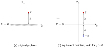
The image principle. (a) A point charge q at height h above an infinite grounded conducting plane. (b) The plane removed and replaced by an image charge -q at the mirror point. In the region y>0 both problems have the same potential. — **Figure 3.4.19.** The image principle. (a) A point charge $q$ at height $h$ above an infinite grounded conducting plane. (b) The plane removed and replaced by an image charge $- q$ at the mirror point. In the region $y > 0$ both problems have the same potential.

Place the plane at $y = 0$ and the charge at $(0, h, 0)$ . Whatever the induced charge is, the potential in the region $y > 0$ must satisfy four conditions:

The potential is zero everywhere on the grounded plane: $V (x, 0, z) = 0$ .
At points very close to $q$ the potential approaches that of the point charge alone, $V \to q / (4 π ε_{0} R)$ , where $R$ is the distance from $q$ . (The only charge in the region $y > 0$ is $q$ , and near it its own field dominates everything else.)
At points very far away from $q$ the potential approaches zero.
The potential is an even function of $x$ and of $z$ , because the geometry is symmetric with respect to the planes $x = 0$ and $z = 0$ .

It is quite difficult to construct a solution satisfying all of these directly, by integrating Laplace's or Poisson's equation. In some problems, however, there are equivalent sources: a different, simpler arrangement of charges that produces the same potential in the region of interest. Before we use this idea we must make sure that "producing the same potential on the boundaries" really means "producing the same potential everywhere in the region". That is the content of the uniqueness theorem.

The uniqueness theorem

Uniqueness theorem

In a region bounded by conductors held at given potentials (the region may extend to infinity, where $V \to 0$ ), and containing a given distribution of free charge, there is only one potential that satisfies Poisson's equation and these boundary conditions.

In plain words

If two potentials obey the same equation, with the same charges, inside the same region and agree on its whole boundary, they are the same potential. The boundary values and the charges inside completely fix the field, just as a soap film is completely fixed by the wire frame it hangs on.

The practical meaning is liberating: however we find a potential that satisfies Poisson's equation in the region and the boundary conditions, it is the solution. Guessing is allowed, provided we check the guess.

The image solution

Let us try the free-space potential of $q$ at $(0, h, 0)$ together with an image charge $- q$ at the mirror point $(0, - h, 0)$ , Figure 3.4.19(b):

V (x, y, z) R_{1} R_{2} = \frac{q}{4 π ε _{0}} (\frac{1}{R _{1}} - \frac{1}{R _{2}}), = x^{2} + (y - h)^{2} + z^{2}, = x^{2} + (y + h)^{2} + z^{2} . (3.4.20)

We check the four conditions.

On $y = 0$ , $R_{1} = R_{2} = x^{2} + h^{2} + z^{2}$ , hence $V = 0$ . $✓$
Near $q$ , $R_{1} \to 0$ while $R_{2} \to 2 h$ , so the first term dominates and $V \to q / (4 π ε_{0} R_{1})$ . $✓$
When $R_{1}, R_{2} \to \infty$ , $V \to 0$ . $✓$
$V$ depends on $x$ and $z$ only through $x^{2}$ and $z^{2}$ . $✓$

Moreover, the potential (3.4.20) satisfies Poisson's equation in the region $y > 0$ with the correct charge there: the only charge in this region is $q$ , the image lying outside it. By the uniqueness theorem, Eq. (3.4.20) is the solution for $y > 0$ . Below the plane, inside the conductor, the real field is zero. The image charge is a mathematical device, not a physical charge, and the equivalent problem tells us nothing about the region $y < 0$ . The field above the plane follows by differentiation, or directly from Coulomb's law for the two charges:

Point charge above a grounded plane

E = - \nabla V = \frac{q}{4 π ε _{0}} (\frac{R _{1}}{R _{1}^{3}} - \frac{R _{2}}{R _{2}^{3}}) (y > 0), (3.4.21)

R_{1} R_{2} = x a_{x} + (y - h) a_{y} + z a_{z}, = x a_{x} + (y + h) a_{y} + z a_{z} .

The image method as “before and after”, both computed: field lines (orange) and equipotentials (blue). (a) The real problem: every field line leaves q and ends perpendicularly on the plane, where it meets the induced negative charge. Below the plane, in the metal, there is no field. (b) The equivalent problem: the plane is removed and the image -q placed at the mirror point. In the upper half the two pictures are identical line for line, which is the content of the uniqueness theorem. The lower half of (b) is a fiction that we never use. Here: (a) real problem: q above a grounded metal plane. — **Figure 3.4.20.** The image method as “before and after”, both computed: field lines (orange) and equipotentials (blue). (a) The real problem: every field line leaves $q$ and ends perpendicularly on the plane, where it meets the induced negative charge. Below the plane, in the metal, there is no field. (b) The equivalent problem: the plane is removed and the image $- q$ placed at the mirror point. In the upper half the two pictures are identical line for line, which is the content of the uniqueness theorem. The lower half of (b) is a fiction that we never use. Here: (a) real problem: $q$ above a grounded metal plane.

(b) Equivalent problem: q and its image -q. — (b) Equivalent problem: $q$ and its image $- q$ .

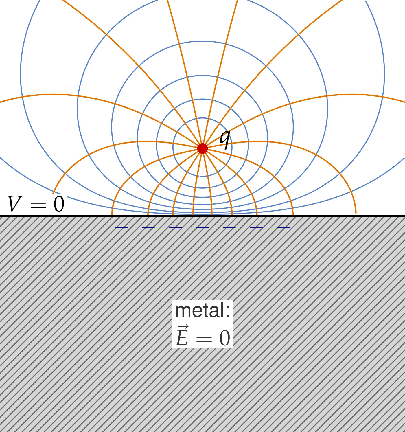
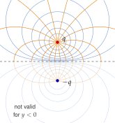
Figure 3.4.20 shows the result. The field lines start on $q$ and all end on the plane, at right angles to it. This is precisely the behaviour required by the conductor condition $E_{τ} = 0$ .

The numerical solver below starts from the same arrangement: solve it and compare the computed field lines and equipotentials with Figure 3.4.20(a), then move the charge and watch the lines still meet the grounded plane at right angles.

InteractiveLoading simulation…

Induced surface charge and the force on the charge

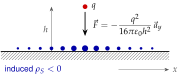
Left: the induced surface charge density on the plane, normalised to its value under the charge, and the fraction of the total induced charge -q found within a distance x of the foot of the perpendicular. Right: the induced charge is negative and concentrated under q, and q is attracted towards the plane. — **Figure 3.4.21.** Left: the induced surface charge density on the plane, normalised to its value under the charge, and the fraction of the total induced charge $- q$ found within a distance $x$ of the foot of the perpendicular. Right: the induced charge is negative and concentrated under $q$ , and $q$ is attracted towards the plane.

Induced negative charge concentrated under q and the attractive force on q

On the plane, at a distance $x$ from the foot of the perpendicular from $q$ (by symmetry we may take the point on the $x$ -axis, $z = 0$ ), the two distances are equal, $R_{1} = R_{2} = x^{2} + h^{2}$ , and $R_{1} - R_{2} = - 2 h a_{y}$ . The tangential components of the two Coulomb fields cancel and the normal components add:

E (x, 0, 0) = \frac{q}{4 π ε _{0}} \frac{R _{1} - R _{2}}{( x ^{2} + h ^{2} ) ^{3/2}} = - \frac{q}{4 π ε _{0}} \frac{2 h}{( x ^{2} + h ^{2} ) ^{3/2}} a_{y} .

The normal pointing out of the conductor into the region $y > 0$ is $a_{n} = a_{y}$ , and the conductor condition $ρ_{S} = ε_{0} E_{n}$ gives the induced surface charge density

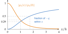
ρ_{S} (x) = ε_{0} E_{y} (x, 0, 0) = - \frac{q h}{2 π ( x ^{2} + h ^{2} ) ^{3/2}} [C/ m^{2}] . (3.4.22)

It has the opposite sign to $q$ , is largest directly under the charge, $ρ_{S} (0) = - q / (2 π h^{2})$ , and decreases quickly: $ρ_{S} (h) = 2^{- 3/2} ρ_{S} (0) = 0.35 ρ_{S} (0)$ (Figure 3.4.21).

Total induced charge

We add up the charge on rings of radius $x$ and width $d x$ around the foot, of area $2 π x d x$ :

Q_{ind} = \int_{0}^{\infty} ρ_{S} (x) 2 π x d x = - q h \int_{0}^{\infty} \frac{x d x}{( x ^{2} + h ^{2} ) ^{3/2}} = - q h [\frac{- 1}{x ^{2} + h ^{2}}]_{0}^{\infty} = - q h \cdot \frac{1}{h} = - q .

The plane carries exactly the charge of the image: every field line that leaves $q$ ends on the plane. Within a radius $a$ the same integral gives $(1 - h / a^{2} + h^{2}) (- q)$ : $29 %$ of the induced charge lies within $a = h$ , one half within $a = 3 h$ .

Force on q

The force on $q$ is exerted by the induced charge on the plane. In the region $y > 0$ the field of the induced charge is the field of the image (that is what the equivalence means), so at the position of $q$ we may use the image:

F = q E_{image} = - \frac{q ^{2}}{4 π ε _{0} ( 2 h ) ^{2}} a_{y} = - \frac{q ^{2}}{16 π ε _{0} h ^{2}} a_{y} [N] . (3.4.23)

The force is always attractive, whatever the sign of $q$ : a charge is always pulled towards a grounded conducting plane. For $q = 1$ nC at $h = 1$ cm in air, $F = 9 \times 1 0^{9} \times 1 0^{- 18} / (4 \times 1 0^{- 4}) = 22.5$ μN. The energy of the arrangement is not that of two real charges $2 h$ apart. To pull $q$ to infinity we integrate the force while the image moves together with $q$ : $W = \int_{h}^{\infty} q^{2} / (16 π ε_{0} y^{2}) d y = q^{2} / (16 π ε_{0} h)$ , which is half of $q^{2} / (8 π ε_{0} h)$ , because there is no field below the plate in which energy could be stored. The earth is a good conductor and acts as such a grounded plane for static and power-frequency fields, so the same method describes a charged object or a charged overhead wire above the ground.

ρ_{S} (x) = - \frac{q h}{2 π ( x ^{2} + h ^{2} ) ^{3/2}}, Q_{ind} = - q, F = \frac{q ^{2}}{16 π ε _{0} h ^{2}}

Move the charge up and down above the grounded plane in the tool below: the image follows it, the induced charge spreads out as $h$ grows but always adds up to $- q$ , and the attraction falls as $1/ h^{2}$ .

InteractiveLoading simulation…

The same construction works for a charged overhead wire above the ground: change the height of the line charge in the tool below and watch the field lines of the wire and its image end perpendicularly on the ground, and the field at ground level grow as the wire comes closer.

InteractiveLoading simulation…

Recipe · The image method

Mark the region of interest (where we want the field) and the conductor surfaces that bound it, with their potentials.
Remove the conductors. Place image charges outside the region of interest so that, together with the real charges, they give the required potential on every boundary. For a grounded plane: the same distance on the other side, the opposite sign.
Check: inside the region only the real charges remain (so Poisson's equation is unchanged), and every boundary condition is met. The uniqueness theorem then guarantees the answer.
Compute $V$ and $E$ in the region from all charges, real and image.
On the conductor, $ρ_{S} = ε E_{n}$ gives the induced charge, and the force on a real charge is the force exerted by the images.
Never use the equivalent problem outside the region of interest.

Common mistake · Image on the wrong side, with the wrong sign, or used in the wrong region

The image of $q$ in a grounded plane is $- q$ , at the mirror point behind the plane. It is not $+ q$ , and it is not on the same side as $q$ (an image inside the region of interest would change Poisson's equation there). The image field is valid only in front of the plane. Behind it, in the metal, $E = 0$ . And the image is not a real charge: the energy is not that of two real charges $2 h$ apart.

Quick check

A charge of $- 2$ nC is $3$ cm above a large grounded metal plate. Where is its image, what is its charge, and how large is the force?

The image is $+ 2$ nC, $3$ cm below the surface of the plate. The force is attractive, $F = q^{2} / (16 π ε_{0} h^{2}) = 9 \times 1 0^{9} \times (2 \times 1 0^{- 9})^{2} / (4 \times 0.0 3^{2}) = 10$ μN.

3.4.8 The image principle

The problem

The uniqueness theorem

The image solution

Induced surface charge and the force on the charge

Total induced charge

Force on q