Electromagnetic Fields and Waves: Notes, Solved Problems and Interactive Lab

3.3 Electrostatic Potential

The electrostatic potential V turns Coulomb's vector integral into one scalar integral, gives the field as E = −∇V, the work as q(V_B − V_A) and, through Poisson's and Laplace's equations, the potential between conductors whose voltages are known.

24 solved examples and exercises6 interactive tools

In this section you will learn

what the electrostatic potential $V$ is, and why this single scalar function contains the whole electric field, $E = - \nabla V$ ,
how to compute $V$ in two ways: by adding up the contributions of the charges, and by integrating a known field from a reference point,
why the work done on a charge does not depend on the path, and what the first fundamental equation $\nabla \times E = 0$ means,
how to read equipotential surfaces like the contour lines of a map, with $E$ pointing "downhill",
how Poisson's and Laplace's equations give the potential when the voltages of conductors, rather than the charges, are known, and
where volts meet engineering: electron guns and the electron volt, and the touch and step voltage around an earth electrode.

Think of a ball on a hilly landscape (Figure 3.3.1). To roll it uphill from a point A to a point B you must do work, and that work is $m g (h_{B} - h_{A})$ : it depends only on the two heights, not on whether you push the ball straight up the slope or along a long, winding road. Gravity always pulls the ball downhill, along the steepest descent, which on a map is perpendicular to the contour lines. A single number per point, the height, tells you everything: where the ball will roll, how hard it is pulled, and how much energy it costs to move it.

The picture behind this whole section. (a) Lifting a ball from A to B costs mg(h_B-h_A). (b) On the contour map the straight trail and the winding trail from A (50 m) to B (300 m) cost the same work, because they start and end at the same heights. The downhill direction -\bm{\nabla} h is perpendicular to the contour lines. In electrostatics the height is replaced by the potential V, the contour lines by equipotential surfaces and the downhill direction by the field \vec E=-\bm{\nabla} V. — **Figure 3.3.1.** The picture behind this whole section. (a) Lifting a ball from A to B costs $m g (h_{B} - h_{A})$ . (b) On the contour map the straight trail and the winding trail from A (50 m) to B (300 m) cost the same work, because they start and end at the same heights. The downhill direction $- \nabla h$ is perpendicular to the contour lines. In electrostatics the height is replaced by the potential $V$ , the contour lines by equipotential surfaces and the downhill direction by the field $E = - \nabla V$ .

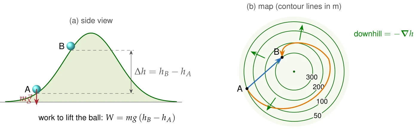
In this section we find that the electrostatic field has exactly the same structure. There is a scalar function, the electrostatic potential $V$ , measured in volts, that plays the role of height (Table 3.3.1). The field points "downhill" in $V$ , the work needed to move a charge is the charge times the difference of $V$ , and the surfaces of constant $V$ are the contour lines of an electrical landscape. Engineers almost never talk about fields directly: batteries, power supplies, oscilloscopes and voltmeters all deal in volts. This section explains what a volt is, and why one number per point is enough.

Table 3.3.1. The gravitational analogy used throughout this section (near the ground, $g$ constant).

	gravity	electrostatics
what is moved	mass $m$	charge $q$
"height" (potential energy per unit)	$g h [J/kg]$	$V [V = J/C]$
potential energy	$m g h$	$q V$
force	$- m \nabla (g h) = m g$	$- q \nabla V = q E$
work to move from A to B	$m g (h_{B} - h_{A})$	$q (V_{B} - V_{A})$
lines of constant "height"	contour lines	equipotential surfaces
zero level	sea level (a convention)	reference point (a convention)

3.3 Electrostatic Potential

Contents of Section 3.3

Problems · 3

Home exercises · 9

Further exercises · 10

Worked examples · 2