Electromagnetic Fields and Waves: Notes, Solved Problems and Interactive Lab

From Coulomb's law to a scalar function

According to Coulomb's law and the superposition principle (Section 3.1), the electric field produced at a field point $P (x, y, z)$ by a volume charge density $ρ_{v}$ filling a region $V$ is

E (x, y, z) = \frac{1}{4 π ε _{0}} ∭_{V} \frac{ρ _{v} ( x ^{'} , y ^{'} , z ^{'} ) R}{R ^{3}} \times d x^{'} d y^{'} d z^{'} [V/m], (3.3.1)

where $R = r - r^{'}$ is the displacement vector from the source point $Q (x^{'}, y^{'}, z^{'})$ to the field point $P$ , and $R = ∣ R ∣$ . (Primed coordinates always belong to the source, unprimed ones to the field point.) This formula is complete (in principle every electrostatic field can be computed with it), but it is laborious. The integrand is a vector whose direction changes from one source point to the next, so Eq. (3.3.1) is really three scalar integrals, one for each component, and in most problems a good part of the work consists of showing that some of them cancel.

We now show that the whole vector field can be generated from one scalar integral. The plan has three steps: (1) find the gradient of the simple function $1/ R$ , (2) recognise that gradient inside the integrand of Eq. (3.3.1), and (3) move the gradient outside the integral.

Step 1: a useful identity

Consider $1/ R$ as a function of the field-point coordinates $(x, y, z)$ , with the source point Q held fixed. Since

R = [(x - x^{'})^{2} + (y - y^{'})^{2} + (z - z^{'})^{2}]^{1/2},

the chain rule gives

\frac{\partial}{\partial x} (\frac{1}{R}) = d (1/ R) / d R - \frac{1}{R ^{2}} \frac{\partial R}{\partial x} = - \frac{1}{R ^{2}} \cdot \partial R / \partial x \frac{2 ( x - x ^{'} )}{2 R} = - \frac{x - x ^{'}}{R ^{3}},

and in the same way $\partial (1/ R) / \partial y = - (y - y^{'}) / R^{3}$ and $\partial (1/ R) / \partial z = - (z - z^{'}) / R^{3}$ . Collecting the three components into a vector,

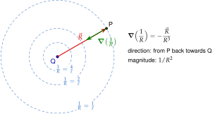
\nabla (\frac{1}{R}) = - \frac{1}{R ^{3}} [(x - x^{'}) a_{x} + (y - y^{'}) a_{y} + (z - z^{'}) a_{z}] = - \frac{R}{R ^{3}} . (3.3.2)

The gradient here acts on the unprimed coordinates. The result has a simple picture (Figure 3.3.2): $1/ R$ is constant on spheres centred at Q and grows as we approach Q. Its gradient therefore points straight back towards Q, i.e. along $- R$ , and its magnitude is the rate of change $∣ d (1/ R) / d R ∣ = 1/ R^{2}$ .

The function 1/R is constant on spheres around the source point Q (the dashed circles, drawn for R=\ell/4, \ell/2 and \ell, where \ell is an arbitrary length). It increases fastest when the field point P moves straight towards Q, so its gradient at P points along -\vec R. — **Figure 3.3.2.** The function $1/ R$ is constant on spheres around the source point Q (the dashed circles, drawn for $R = ℓ /4$ , $ℓ /2$ and $ℓ$ , where $ℓ$ is an arbitrary length). It increases fastest when the field point P moves straight towards Q, so its gradient at P points along $- R$ .

Step 2: the field as a gradient

Equation (3.3.2) says $R / R^{3} = - \nabla (1/ R) = \nabla (- 1/ R)$ . Substituting this into Eq. (3.3.1) gives

E (x, y, z) = \frac{1}{4 π ε _{0}} ∭_{V} ρ_{v} (x^{'}, y^{'}, z^{'}) \times \nabla (- \frac{1}{R}) d x^{'} d y^{'} d z^{'} .

Step 3: the gradient comes out of the integral

The integration runs over the primed (source) coordinates, while $\nabla$ differentiates with respect to the unprimed (field) coordinates. The charge density $ρ_{v} (x^{'}, y^{'}, z^{'})$ does not depend on $(x, y, z)$ at all, so it behaves like a constant for $\nabla$ . The order of integration and differentiation can therefore be exchanged, and $\nabla$ can be taken outside the integral:

E (x, y, z) = - \nabla [\frac{1}{4 π ε _{0}} ∭_{V} \frac{ρ _{v} ( x ^{'} , y ^{'} , z ^{'} )}{R} \times d x^{'} d y^{'} d z^{'}] . (3.3.3)

The quantity in square brackets is a scalar function of the field point. It deserves a name.

Definition · Electrostatic potential

The electrostatic potential of a volume charge distribution $ρ_{v}$ is

V (x, y, z) = \frac{1}{4 π ε _{0}} ∭_{V} \frac{ρ _{v} ( x ^{'} , y ^{'} , z ^{'} )}{R} \times d x^{'} d y^{'} d z^{'} + V_{0} [V], (3.3.4)

where $V_{0}$ is an arbitrary constant. Its unit is the volt, $1 V = 1 J/C$ .

Since the gradient of a constant is zero, adding $V_{0}$ does not change Eq. (3.3.3), and we arrive at the central relation of this section.

Field and potential

E (x, y, z) = - \nabla V (x, y, z) (3.3.5)

In plain words

The electric field is the "downhill slope" of the potential. $E$ points in the direction in which $V$ decreases fastest, and its magnitude is how many volts $V$ drops per metre in that direction. This is why the unit of the electric field, the newton per coulomb, is usually written volt per metre, V/m.

These two statements are just the meaning of the gradient (Section 2.2): $\nabla V$ points in the direction of the fastest increase of $V$ and its magnitude is that maximum rate of increase. The minus sign turns "fastest increase" into "fastest decrease".

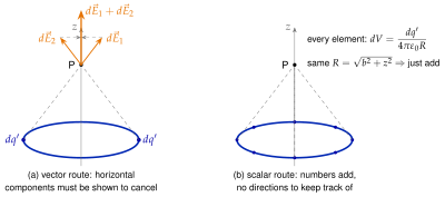
The practical gain is considerable. Instead of three integrals with vector integrands we evaluate one integral of a scalar, $ρ_{v} / R$ , in which no unit vectors and no vector cancellations appear. The field then follows by differentiation, which is always easier than integration. Figure 3.3.3 compares the two routes for a charged ring.

Two routes to the field of a charged ring on its axis. (a) Coulomb's law adds vectors: the contributions d\vec E_1 and d\vec E_2 of two opposite elements have horizontal components that cancel, which must be argued element by element. (b) The potential adds numbers: every element is at the same distance R from P, so V=Q/(4\pi\varepsilon_0R) at once, and \vec E=-\bm{\nabla} V follows by one differentiation (Exercise 3.3.1). — **Figure 3.3.3.** Two routes to the field of a charged ring on its axis. (a) Coulomb's law adds vectors: the contributions $d E_{1}$ and $d E_{2}$ of two opposite elements have horizontal components that cancel, which must be argued element by element. (b) The potential adds numbers: every element is at the same distance $R$ from P, so $V = Q / (4 π ε_{0} R)$ at once, and $E = - \nabla V$ follows by one differentiation (Exercise 3.3.1).

Quick check

A thin ring of radius $10 cm$ carries a total charge of $1 nC$ . What is the potential at its centre (with $V = 0$ at infinity)? What is the field there?

Every element of the ring is at the same distance $R = 0.1 m$ from the centre, so $V = Q / (4 π ε_{0} R) = 9 \times 1 0^{9} \times 1 0^{- 9} /0.1 = 90 V$ . The field is zero: the contributions of opposite elements cancel. A zero field does not mean a zero potential.

Potential of point charges and of line, surface and volume charges

The same argument applies to every type of source considered in Section 3.1, and only the charge element $d q^{'}$ changes. For a point charge $q$ at $Q$ the Coulomb field $q R / (4 π ε_{0} R^{3})$ is, by Eq. (3.3.2), the negative gradient of $q / (4 π ε_{0} R)$ . For $N$ point charges the fields add, and so do the potentials. Summarising (with the reference constant $V_{0}$ chosen as discussed in Section 3.3.2):

Potential of point, line, surface and volume charges

Point charge $q$ at Q:

V (P) = \frac{q}{4 π ε _{0} R} (3.3.6)

$N$ point charges:

V (P) = \frac{1}{4 π ε _{0}} k = 1 \sum N \frac{q _{k}}{R _{k}} (3.3.7)

Line charge:

V (P) = \frac{1}{4 π ε _{0}} \int_{L} \frac{ρ _{L} d l ^{'}}{R} (3.3.8)

Surface charge:

V (P) = \frac{1}{4 π ε _{0}} \iint_{S} \frac{ρ _{S} d S ^{'}}{R} (3.3.9)

Volume charge:

V (P) = \frac{1}{4 π ε _{0}} ∭_{V} \frac{ρ _{v} d v ^{'}}{R} (3.3.10)

All five are special cases of one rule, $V (P) = \frac{1}{4 π ε _{0}} \int d q^{'} / R$ : each charge element contributes $d q^{'} / (4 π ε_{0} R)$ , and the contributions are simply added. Unlike the field, the potential of a point charge does not depend on the direction from Q to P but only on the distance $R$ . Positive charges raise the potential around them, negative charges lower it. Home exercises 3.3.1–3.3.4 and Exercises 3.3.1–3.3.3 compute potentials of lines, rings, disks and spherical shells in this way and then differentiate them to obtain the fields. Comparing them with the direct integrations of Section 3.1 (Home exercise 3.1.1, Problems 3.1.2 and 3.1.3) shows how much simpler the scalar route is.

Recipe · Finding

V

by superposition of charges

Sketch the charges and the field point P. Choose coordinates that fit the source (e.g. cylindrical for a disk).
Write the charge element $d q^{'} = ρ_{L} d l^{'}$ , $ρ_{S} d S^{'}$ or $ρ_{v} d v^{'}$ , including the Jacobian ( $ρ^{'} d ϕ^{'} d ρ^{'}$ , $r^{'2} sin θ^{'} d r^{'} d θ^{'} d ϕ^{'}$ , …).
Write the distance $R = ∣ r - r^{'} ∣$ from the element to P (a scalar, so no unit vector is needed).
Integrate $d q^{'} / (4 π ε_{0} R)$ over the source. For point charges, add $q_{k} / (4 π ε_{0} R_{k})$ with signs.
If the field is wanted, take $E = - \nabla V$ (see the recipe in Section 3.3.4).
Check: far from a finite source, $V \to Q_{total} / (4 π ε_{0} r)$ .

Common mistake

Using $1/ R^{2}$ instead of $1/ R$ (mixing up the potential with the field), or carrying the vector $R$ into the potential integral. The potential needs only the distance $R$ . It has no direction.

Common mistake · Differentiating a potential known only on a line

If $V$ has been computed only on the $z$ -axis, $- d V / d z$ gives only $E_{z}$ there. The other components are zero only if symmetry says so (as on the axis of a ring or a disk). In general the potential must be known in a neighbourhood of P before all components of $E$ can be found from it.

Quick check

Charges $+ q$ and $- q$ sit at $z = \pm d /2$ . What is the potential at the origin? Is the field zero there?

$V = \frac{1}{4 π ε _{0}} (\frac{q}{d /2} - \frac{q}{d /2}) = 0$ . The field is not zero: both charges push and pull a test charge the same way, $E = - a_{z} 2 q / (π ε_{0} d^{2})$ , from $+ q$ towards $- q$ . A zero potential does not mean a zero field.

3.3.1 The electrostatic potential

From Coulomb's law to a scalar function

Step 1: a useful identity

Step 2: the field as a gradient

Step 3: the gradient comes out of the integral

Potential of point charges and of line, surface and volume charges