Section 3.3 · Topic 6 of 8
3.3.6 Applications of the electrostatic potential
The potential turns a vector problem into a scalar one: one number per point, from which recovers the field and the energy exchanged with a charge. It is also the quantity a voltmeter measures, so most practical statements about static fields are in fact statements about volts. The two applications of this subsection (Figure 3.3.18) each rest on one formula of this section: the work–voltage relation and Laplace's equation in a conducting medium. Table 3.3.3 at the end of the subsection lists where each one is worked out with numbers.


Energy = charge × voltage
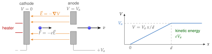
By Eq. (3.3.11) the work done on a charge between two points is fixed by the potential difference, whatever the path. Consider an electron (charge ) released at rest from a heated cathode at potential and accelerated towards an anode at (Figure 3.3.19). The work done by the field on the electron is the negative of the work an external agent would have to do, , and it all goes into kinetic energy:
Only the potential difference matters: the shapes of the electrodes determine the trajectory and the focusing of the beam, but not the final speed. Between plane electrodes a distance apart the potential rises linearly, , and the field is uniform (Problem 3.3.1). It points from the anode to the cathode, and the force on the electron points towards the anode. A negative charge "rolls uphill" in : for it, the landscape is turned upside down.
The electron volt
The energy an electron gains when it passes through a potential difference of one volt is called one electron volt:
A 25 kV tube produces 25 keV electrons: in this unit the energy is the accelerating voltage. Typical accelerating voltages are about 25 kV in a colour cathode-ray tube, 1–30 kV in a scanning electron microscope, 80–300 kV in a transmission electron microscope and 30–150 kV in a medical X-ray tube. In an X-ray tube the whole energy of one electron can be converted into a single photon, so the shortest emitted wavelength is (the Duane–Hunt law). For this is about 12 pm.
Raise the accelerating voltage and note that the electron arrives faster but is deflected less by the same plate voltage: the transit time between the plates shrinks.
An electron starts at rest at a point at and arrives at a point at . How much kinetic energy has it gained, in eV and in J? Would a proton gain energy on the same trip?
. A proton (charge ) would lose on that trip. In fact it cannot make it at all if it starts at rest, because for a positive charge the point at is "uphill".
At 1 kV the electron already reaches , about 6 % of the speed of light, and crosses a 2 cm gap in about 2 ns (Worked example 3.3.1). Above a few tens of kilovolts the classical formula (3.3.18) overestimates the speed (by 3.6 % at 25 kV and by about 14 % at 100 kV), and the relativistic expression , with , must be used. The energy itself, however, is exact at any voltage, which is why particle energies are quoted in electron volts.
E = −∇V under our feet
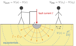
When a fault current flows into the ground through an earth electrode, it spreads out through the soil. In this application denotes the resistivity of the soil (typically 10–1000 m), not a charge density. In the soil the current density and the field are related by Ohm's law, . In steady state no charge accumulates anywhere in the (homogeneous) soil, so , hence , and with :
The potential in the soil obeys Laplace's equation again, and the solutions of Problems 3.3.1–3.3.3 apply. (A steady current field is curl-free just like an electrostatic one, so the potential concept carries over unchanged.)
For a hemispherical electrode of radius the current leaves radially and crosses hemispheres of area , so and
with remote earth as the reference, . This is the solution of Laplace's equation found in Problem 3.3.3.
Definitions
The quantities used in earthing design follow directly from Eq. (3.3.19) (Figure 3.3.20):
- the earth potential rise , the voltage of the electrode and of everything bonded to it with respect to remote earth, which during a fault can reach tens of kilovolts (the ratio is the resistance of the electrode),
- the touch voltage , which appears across the body of a person whose hand is on the earthed structure while the feet stand at distance , and
- the step voltage , which appears between the two feet, about one metre apart, of a person standing at distance .
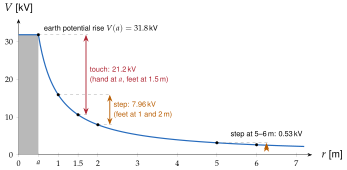
Both the touch and the step voltage are largest where is largest, i.e. next to the electrode. For , m and the electrode rises to 31.8 kV. A person touching it with the feet 1 m from its edge () is exposed to 21.2 kV, and a person merely standing with the feet at and from its centre to 7.96 kV between the feet, falling to 0.53 kV for –6 m (Worked example 3.3.2). Figure 3.3.21 reads these numbers off the potential curve: touch and step voltages are simply vertical distances on it.
Remedy
Standards for substation earthing (such as IEEE Std 80) set limits for both quantities. The remedy is equipotential bonding: a buried earthing mesh under the whole station brings everything a person can touch or stand on to nearly the same potential, i.e. it makes small where people are. A surface layer of high-resistivity crushed rock further limits the current that can flow through the body.
What hurts is not the voltage of the ground but the voltage between the two points the body touches. Earthing design is the art of making the potential landscape flat where people stand.
Table 3.3.3. The applications of this section, the physics they use and where they are worked out.
| Application | Physics used | Worked out in |
|---|---|---|
| 3.3.1 Electron gun | , electron volt | Problem 3.3.1, Worked example 3.3.1 |
| 3.3.2 Earthing | Laplace's equation in soil, | Problem 3.3.3, Worked example 3.3.2 |