Electromagnetic Fields and Waves: Notes, Solved Problems and Interactive Lab

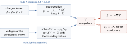
So far the potential has been computed from a known charge distribution. In many engineering problems, however, the charges are not known in advance. What is known are the voltages: a battery or a supply holds two electrodes at fixed potentials, a screen is earthed. The charges arrange themselves on the conductors in a way that is not known beforehand. We need an equation that the potential satisfies at every point of space, which can then be solved with the given potentials as boundary conditions (Figure 3.3.15). It is obtained by combining $E = - \nabla V$ with Gauss's law.

Two routes to the potential. When the charges are known, V is found by adding their contributions. When the voltages of the conductors are known instead, V is found by solving Poisson's or Laplace's equation with those voltages as boundary values. The field and the charges on the conductors then follow from V. — **Figure 3.3.15.** Two routes to the potential. When the charges are known, $V$ is found by adding their contributions. When the voltages of the conductors are known instead, $V$ is found by solving Poisson's or Laplace's equation with those voltages as boundary values. The field and the charges on the conductors then follow from $V$ .

Derivation

We need three short steps: Gauss's law in differential form, the substitution $E = - \nabla V$ , and the definition of the Laplacian. Gauss's law (Section 3.2) states $\nabla \cdot D = ρ_{v}$ , and in free space $D = ε_{0} E$ . Substituting $E = - \nabla V$ step by step,

\nabla \cdot D = ρ_{v} \Rightarrow \nabla \cdot E = \frac{ρ _{v}}{ε _{0}} \Rightarrow \nabla \cdot (- \nabla V) = \frac{ρ _{v}}{ε _{0}} \Rightarrow \nabla \cdot (\nabla V) = - \frac{ρ _{v}}{ε _{0}} .

The divergence of the gradient is the Laplacian (Section 2.2), $\nabla \cdot (\nabla V) = \nabla^{2} V \equiv Δ V$ , which in Cartesian coordinates reads

Δ V = \frac{\partial ^{2} V}{\partial x ^{2}} + \frac{\partial ^{2} V}{\partial y ^{2}} + \frac{\partial ^{2} V}{\partial z ^{2}} .

This gives Poisson's equation. In a region where there is no charge, $ρ_{v} = 0$ , it reduces to Laplace's equation.

Poisson's and Laplace's equations

Δ V = - \frac{ρ _{v}}{ε _{0}} (Poisson’s equation), Δ V = 0 (Laplace’s equation) . (3.3.15)

In plain words

The Laplacian compares the value of $V$ at a point with the average of $V$ on a small sphere around it: for a sphere of radius $h$ , the average is $V + \frac{h ^{2}}{6} Δ V$ (plus terms of order $h^{4}$ ). Laplace's equation therefore says: in empty space, $V$ at every point equals the average of its surroundings. Poisson's equation says that a positive charge density makes $V$ larger than its surroundings (a little hill), and a negative one makes a little pit.

For problems with cylindrical or spherical symmetry the Laplacian is needed in the other two coordinate systems (Section 2.3):

Δ V = \frac{1}{ρ} \frac{\partial}{\partial ρ} (ρ \frac{\partial V}{\partial ρ}) + \frac{1}{ρ ^{2}} \frac{\partial ^{2} V}{\partial ϕ ^{2}} + \frac{\partial ^{2} V}{\partial z ^{2}} (cylindrical), (3.3.16)

Δ V = \frac{1}{r ^{2}} \frac{\partial}{\partial r} (r^{2} \frac{\partial V}{\partial r}) + \frac{1}{r ^{2} sin θ} \frac{\partial}{\partial θ} (sin θ \frac{\partial V}{\partial θ}) + \frac{1}{r ^{2} sin ^{2} θ} \frac{\partial ^{2} V}{\partial ϕ ^{2}} (spherical) . (3.3.17)

What the equations say and how they are used

A local law

Poisson's equation is the differential (point-by-point) counterpart of the integral formula (3.3.4): it relates the curvature of the potential at a point to the charge density at that same point, while Eq. (3.3.4) adds up the contributions of all charges. In fact the integral $\frac{1}{4 π ε _{0}} \int ρ_{v} d v^{'} / R$ is precisely the solution of Poisson's equation that vanishes at infinity. A first check: the potential $q / (4 π ε_{0} r)$ of a point charge must satisfy Laplace's equation everywhere except at the charge itself, and indeed, by Eq. (3.3.17),

Δ (\frac{1}{r}) = \frac{1}{r ^{2}} \frac{d}{d r} (r^{2} \cdot (- \frac{1}{r ^{2}})) = \frac{1}{r ^{2}} \frac{d}{d r} (- 1) = 0 (r \neq = 0) .

Boundary-value problems

In a charge-free region bounded by conductors at given potentials, the potential is found by solving Laplace's equation with those potentials prescribed on the boundaries. It can be shown that this problem has only one solution (the uniqueness theorem), so a solution found by any means (a symmetry argument, an educated guess, a direct integration) is the solution. Once $V$ is known, $E = - \nabla V$ gives the field, and the boundary condition $ρ_{S} = D_{n}$ at each conductor surface gives the charges that the voltages have put on the conductors. Figure 3.3.16 shows a typical two-dimensional example, solved numerically. Problems 3.3.1–3.3.3 are the three simplest cases, in which $V$ depends on one coordinate only: $x$ between parallel plates, $ρ$ between coaxial cylinders and $r$ between concentric spheres (Table 3.3.2). Exercise 3.3.9 adds the case in which $V$ depends on $ϕ$ only.

A boundary-value problem: a long earthed trough (cross-section 3\times2 units) closed by a lid at 100 V, insulated from the walls. Laplace's equation was solved numerically on a fine grid, by requiring each grid value to be the average of its four neighbours. Shown are the computed equipotentials (blue, labels in volts) and field lines (orange) from the lid to the walls. The largest and smallest values of V occur on the boundary, not inside. At the centre V\approx38 V. — **Figure 3.3.16.** A boundary-value problem: a long earthed trough (cross-section $3 \times 2$ units) closed by a lid at $100$ V, insulated from the walls. Laplace's equation was solved numerically on a fine grid, by requiring each grid value to be the average of its four neighbours. Shown are the computed equipotentials (blue, labels in volts) and field lines (orange) from the lid to the walls. The largest and smallest values of $V$ occur on the boundary, not inside. At the centre $V \approx 38$ V.

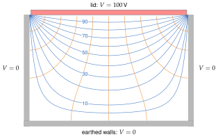
The same trough can be solved live: change the lid voltage and the grid, and watch the solver relax every grid value towards the average of its neighbours until Laplace's equation holds.

InteractiveLoading simulation…

Table 3.3.2. Laplace's equation when $V$ depends on one coordinate only (Problems 3.3.1–3.3.3, Exercise 3.3.9). $A$ and $B$ are fixed by the two boundary values.

geometry	reduced equation	general solution	field
parallel plates, $V (x)$	$\frac{d ^{2} V}{d x ^{2}} = 0$	$V = A x + B$	$E_{x} = - A$ (uniform)
coaxial cylinders, $V (ρ)$	$\frac{1}{ρ} \frac{d}{d ρ} (ρ \frac{d V}{d ρ}) = 0$	$V = A ln ρ + B$	$E_{ρ} = - A / ρ$
concentric spheres, $V (r)$	$\frac{1}{r ^{2}} \frac{d}{d r} (r^{2} \frac{d V}{d r}) = 0$	$V = A / r + B$	$E_{r} = A / r^{2}$
wedge, $V (ϕ)$	$\frac{1}{ρ ^{2}} \frac{d ^{2} V}{d ϕ ^{2}} = 0$	$V = A ϕ + B$	$E_{ϕ} = - A / ρ$

Recipe · Solving a one-dimensional Laplace problem

Check that the region between the conductors contains no charge (otherwise use Poisson's equation).
Use the symmetry to decide which single coordinate $V$ depends on, and drop all other derivatives from the Laplacian in that coordinate system.
Integrate the ordinary differential equation twice, keeping the two constants $A$ , $B$ .
Impose the two boundary values (the potentials of the conductors) and solve for $A$ and $B$ .
Take $E = - \nabla V$ . Then compute $ρ_{S} = D \cdot a_{n}$ on each conductor, with $a_{n}$ pointing out of the conductor into the field region, and $Q = \int ρ_{S} d S$ .
Check: the boundary values are reproduced, $E$ points from high to low $V$ , and the charges on the two conductors are equal and opposite.

Common mistake · The Laplacian in cylindrical or spherical coordinates

Writing $d^{2} V / d ρ^{2} = 0$ for the coaxial problem gives $V = A ρ + B$ , which is wrong. The radial part of the Laplacian is $\frac{1}{ρ} \frac{d}{d ρ} (ρ \frac{d V}{d ρ})$ (cylindrical) or $\frac{1}{r ^{2}} \frac{d}{d r} (r^{2} \frac{d V}{d r})$ (spherical). Only in Cartesian coordinates is it a plain second derivative.

Common mistake

Applying Laplace's equation in a region that contains charge (e.g. inside a charged ball or the depletion layer of a diode). Laplace's equation holds only where $ρ_{v} = 0$ . Elsewhere use Poisson's equation.

No maxima or minima in empty space

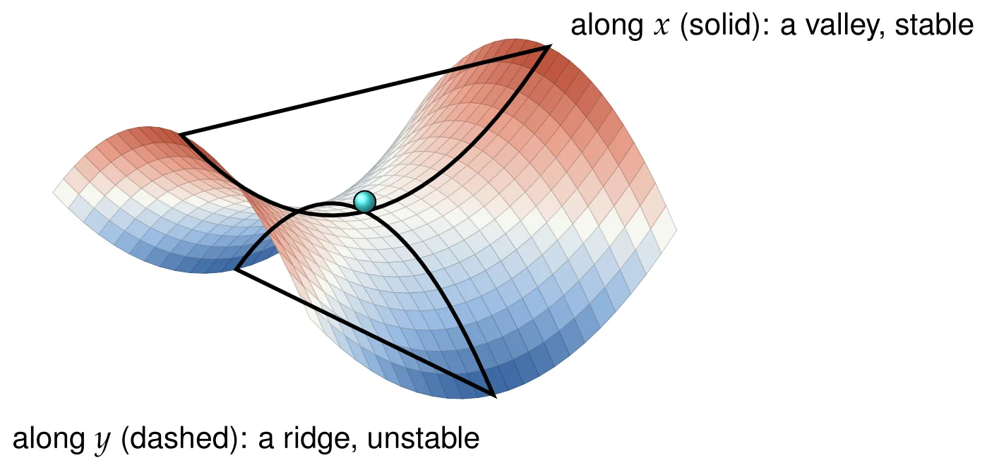
In one dimension Laplace's equation, $d^{2} V / d x^{2} = 0$ , allows only straight lines: the potential has no peak or dip between its boundary values. In three dimensions $Δ V = 0$ says that the three curvatures $\partial^{2} V / \partial x^{2}$ , $\partial^{2} V / \partial y^{2}$ , $\partial^{2} V / \partial z^{2}$ add up to zero, so they cannot all be negative (a maximum) or all positive (a minimum). The averaging property says the same thing: a value that is the average of its surroundings cannot be larger (or smaller) than all of them. Hence in a charge-free region the potential has no local maximum or minimum, and its extreme values are attained on the boundaries (Figure 3.3.16). A charged particle therefore cannot be held in stable equilibrium by electrostatic forces alone (Earnshaw's theorem): at best the potential has a saddle (Figure 3.3.17). Exercise 3.3.5 shows the two-dimensional version of this for an electrostatic quadrupole lens.

The potential V\propto x^2-y^2 near the axis of a quadrupole lens (Exercise 3.3.5) satisfies Laplace's equation. It curves up along x and down along y: the centre is a saddle, not a minimum. A positive charge placed there is pushed back along x but escapes along y. No electrostatic arrangement can trap it in all directions at once. — **Figure 3.3.17.** The potential $V \propto x^{2} - y^{2}$ near the axis of a quadrupole lens (Exercise 3.3.5) satisfies Laplace's equation. It curves up along $x$ and down along $y$ : the centre is a saddle, not a minimum. A positive charge placed there is pushed back along $x$ but escapes along $y$ . No electrostatic arrangement can trap it in all directions at once.

Charge from the potential

Read backwards, Poisson's equation gives the charge density when the potential is known: $ρ_{v} = - ε_{0} Δ V$ (Home exercise 3.3.7, Exercises 3.3.5 and 3.3.6).

Quick check

In some region the potential is $V = 5 x^{2}$ [V, with $x$ in m]. Is the region free of charge?

No: $Δ V = d^{2} (5 x^{2}) / d x^{2} = 10 V/ m^{2}$ , so $ρ_{v} = - ε_{0} Δ V = - 10 ε_{0} \approx - 8.84 \times 1 0^{- 11} C/ m^{3}$ . A uniform negative charge density makes $V$ curve upwards, forming a pit.

Remark

In a dielectric material $ε_{0}$ is replaced by the permittivity $ε$ of the material, $Δ V = - ρ_{v} / ε$ (Section 3.4). In a conducting medium carrying steady currents, $\nabla \cdot J = 0$ leads again to Laplace's equation (Application 3.3.2).

3.3.5 Laplace's and Poisson's equations