Section 3.3 · Further exercises · 2 of 10
Exercise 3.3.2: Two point charges: exact potential and dipole limit
About the further exercises of Section 3.3
The following exercises use only the relations collected at the beginning of this subsection. Exercises 3.3.1–3.3.4 compute potentials from the charge distribution, Exercises 3.3.5–3.3.7 work from the field or the potential, and Exercises 3.3.8–3.3.10 solve Laplace's and Poisson's equations.
Two point charges: exact potential and dipole limit
#cf. Home exercise 3.3.5
Point charges and are located at and .
(a) Write the exact potential at .
(b) Show that for it becomes , and find from it.
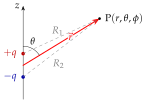
Superposition of two point-charge potentials, with the distances from the law of cosines, then a first-order binomial expansion for , and finally the gradient in spherical coordinates.
By superposition of the two point-charge potentials,
where the distances from to P follow from the law of cosines (the angle between and the -axis is , that between and the -axis is ).
For , neglect against and use for :
The field follows from the gradient in spherical coordinates,
with , and :
changes sign when (swapping the roles of and ), as it must. The unit of is , and , one power faster than a single charge.
This is the field of Home exercise 3.3.5 with and , and the result of Home exercise 3.1.4, obtained here with one scalar expansion instead of a vector one. The plane is the surface (Figure 3.3.14b).