Electromagnetic Fields and Waves: Notes, Solved Problems and Interactive Lab

Potential and height

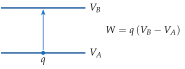
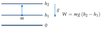
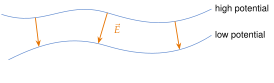
The electrostatic potential plays the role of height in the gravitational field. (a) Charge q lifted between two equipotentials. — **Figure 3.3.8.** The electrostatic potential plays the role of height in the gravitational field. (a) Charge $q$ lifted between two equipotentials.

(b) Mass m lifted between two levels. Lifting a charge from the equipotential V_A to V_B costs q(V_B-V_A), just as lifting a mass from height h_1 to h_2 costs mg(h_2-h_1). In both cases moving along a level costs nothing. — (b) Mass $m$ lifted between two levels. Lifting a charge from the equipotential $V_{A}$ to $V_{B}$ costs $q (V_{B} - V_{A})$ , just as lifting a mass from height $h_{1}$ to $h_{2}$ costs $m g (h_{2} - h_{1})$ . In both cases moving along a level costs nothing.

Equation (3.3.13), $V_{r} = \int_{r}^{\infty} E \cdot d l$ , has a familiar gravitational counterpart (Table 3.3.1). Near the ground the gravitational potential energy of a mass $m$ at height $h$ is $m g h$ , and lifting it from $h_{1}$ to $h_{2}$ costs $m g (h_{2} - h_{1})$ whatever the path. In the same way, carrying a charge $q$ from a point at potential $V_{A}$ to a point at potential $V_{B}$ costs $q (V_{B} - V_{A})$ (Figure 3.3.8). The potential $V$ is the potential energy per unit charge, exactly as $g h$ is the potential energy per unit mass. The "ground level" $h = 0$ is a matter of convention, just like the reference point of $V$ .

Definition · Equipotential surface

An equipotential surface is a surface on which the potential has the same value at every point, $V (x, y, z) = const$ . No work is required to move a charge along an equipotential surface.

The potential landscape

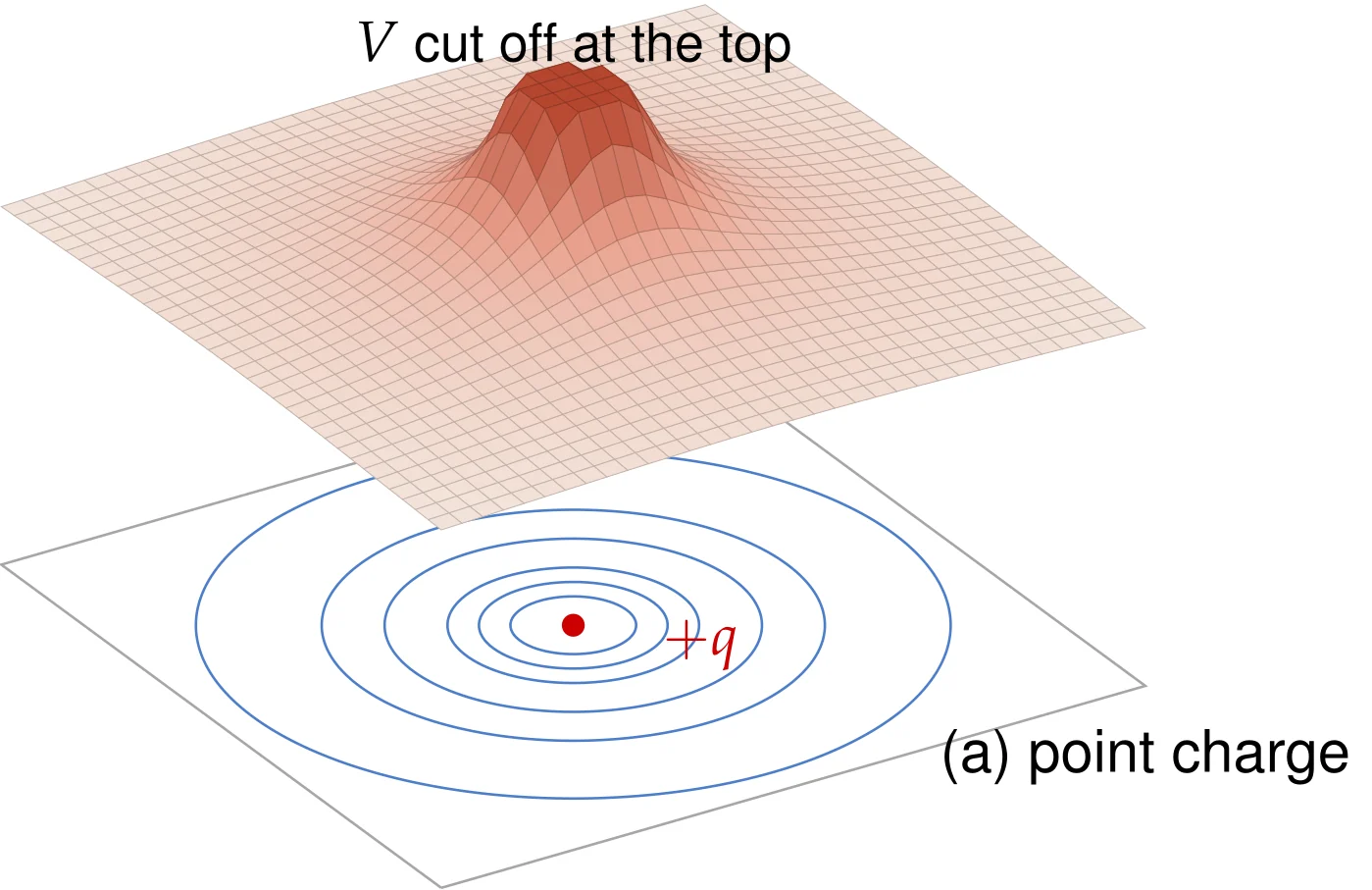
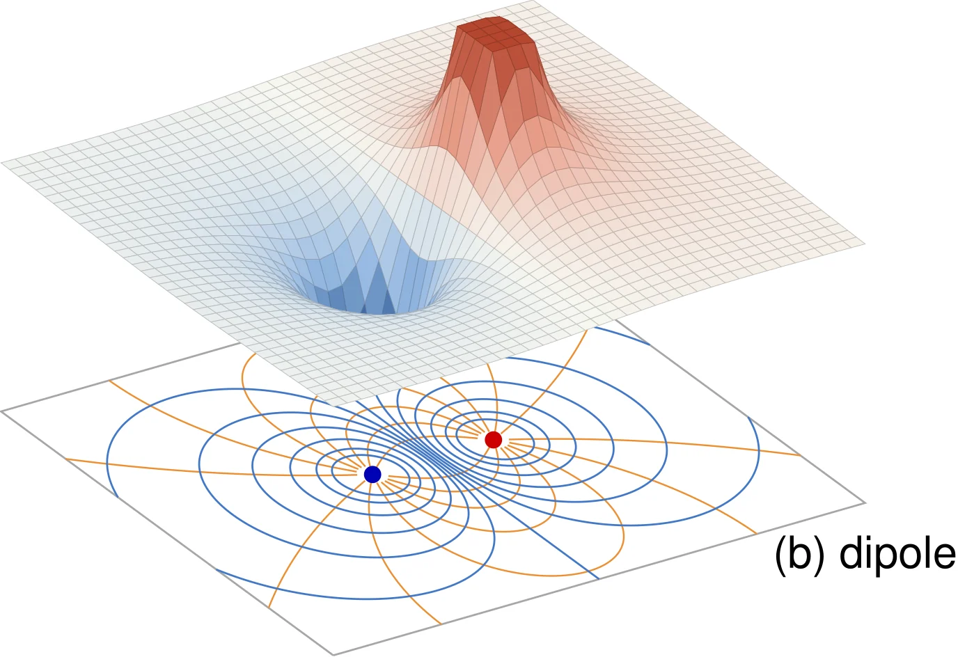
The analogy can be made literal. Take a plane through the charges and plot the potential above each of its points as a height. The result is a landscape (Figure 3.3.9). A positive point charge is a steep mountain, $V \propto 1/ r$ , which rises without limit at the charge. A negative charge is a pit, and a dipole is a mountain next to a pit. The contour lines of the landscape, drawn on the floor of the figure, are the traces of the equipotential surfaces in the plane. A positive test charge placed on the landscape behaves like a ball: it is pushed downhill, from the peak towards the pit.

Potential landscapes over a plane through the charges, with the height (and colour) giving V: (a) a positive point charge, — **Figure 3.3.9.** Potential landscapes over a plane through the charges, with the height (and colour) giving $V$ : (a) a positive point charge,

(b) a dipole, +q (red dot) and -q (blue dot). The surfaces are cut off at |V|=3 units, since V grows without limit at a point charge. On the floor are the computed contour lines of the same functions (the equipotentials, blue) and, in (b), the computed field lines (orange), which run downhill from the peak to the pit and cross every contour at a right angle. — (b) a dipole, $+ q$ (red dot) and $- q$ (blue dot). The surfaces are cut off at $∣ V ∣ = 3$ units, since $V$ grows without limit at a point charge. On the floor are the computed contour lines of the same functions (the equipotentials, blue) and, in (b), the computed field lines (orange), which run downhill from the peak to the pit and cross every contour at a right angle.

Field lines are perpendicular to equipotential surfaces

Let $d l$ be any small displacement within an equipotential surface. Since $V$ does not change along it,

d V = \nabla V \cdot d l = - E \cdot d l = 0.

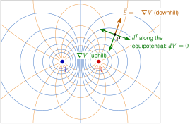
The field is thus perpendicular to every direction tangent to the surface, i.e. field lines cross equipotential surfaces at right angles. Moreover, $E = - \nabla V$ points from high to low potential, and its magnitude is the rate of change of $V$ along the normal $n$ to the surface,

∣ E ∣ = \frac{d V}{d n} ≃ \frac{Δ V}{Δ n} .

If equipotential surfaces are drawn for equal steps $Δ V$ , the field is strong where they are close together and weak where they spread apart (Figures 3.3.10 and 3.3.11).

The computed equipotentials (blue) and field lines (orange) of the dipole of Figure 3.3.9b, seen from above. At the point P the gradient \bm{\nabla} V points uphill, towards the positive charge, and is perpendicular to the equipotential through P, while the field \vec E points the opposite way, downhill. Moving along the equipotential (d\vec l) does not change V. Where the contours crowd together (near the charges) the field is strong. — **Figure 3.3.10.** The computed equipotentials (blue) and field lines (orange) of the dipole of Figure 3.3.9b, seen from above. At the point P the gradient $\nabla V$ points uphill, towards the positive charge, and is perpendicular to the equipotential through P, while the field $E$ points the opposite way, downhill. Moving along the equipotential ( $d l$ ) does not change $V$ . Where the contours crowd together (near the charges) the field is strong.

$Field lines are always perpendicular to the equipotential surfaces and point from high to low potential. Where two equipotentials of given \Delta V come close (centre), the field is strong, and where they are far apart (right), it is weak. (A schematic sketch: each arrow leaves the upper equipotential at a right angle. Computed field lines, which curve so as to meet every equipotential at a right angle, are shown in Figure 3.3.10.)$

Figure 3.3.11. Field lines are always perpendicular to the equipotential surfaces and point from high to low potential. Where two equipotentials of given

Δ V

come close (centre), the field is strong, and where they are far apart (right), it is weak. (A schematic sketch: each arrow leaves the upper equipotential at a right angle. Computed field lines, which curve so as to meet every equipotential at a right angle, are shown in Figure 3.3.10.)

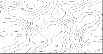
A topographic map is the best everyday picture of these facts (Figure 3.3.12). Its contour lines join points of equal height, i.e. of equal gravitational potential $g h$ . Where the contour lines crowd together the slope $∣ \nabla h ∣$ is steep. Water runs downhill perpendicular to the contour lines, along $- \nabla h$ , just as a positive charge is pushed along $E = - \nabla V$ .

Contour lines of a (synthetic) topographic map join points of equal height, i.e. of equal gravitational potential gh. The labels give the height in metres. The closer the lines, the steeper the slope |\bm{\nabla} h|. Equipotential surfaces of an electrostatic field are the three-dimensional analogue of these lines. — **Figure 3.3.12.** Contour lines of a (synthetic) topographic map join points of equal height, i.e. of equal gravitational potential $g h$ . The labels give the height in metres. The closer the lines, the steeper the slope $∣ \nabla h ∣$ . Equipotential surfaces of an electrostatic field are the three-dimensional analogue of these lines.

Recipe · Getting

E

from

V

Write $V$ in the coordinate system that suits it (Cartesian, cylindrical or spherical).
Take the gradient with the correct scale factors (Section 2.3):

$\nabla V = \frac{\partial V}{\partial x} a_{x} + \frac{\partial V}{\partial y} a_{y} + \frac{\partial V}{\partial z} a_{z} = \frac{\partial V}{\partial ρ} a_{ρ} + \frac{1}{ρ} \frac{\partial V}{\partial ϕ} a_{ϕ} + \frac{\partial V}{\partial z} a_{z} = \frac{\partial V}{\partial r} a_{r} + \frac{1}{r} \frac{\partial V}{\partial θ} a_{θ} + \frac{1}{r s i n θ} \frac{\partial V}{\partial ϕ} a_{ϕ} .$
Put the minus sign in front: $E = - \nabla V$ .
Check: the units are V/m, $E$ points towards lower $V$ , and it is perpendicular to the equipotentials.

Common mistake

Forgetting the scale factors in curvilinear coordinates: writing $E_{θ} = - \partial V / \partial θ$ instead of $E_{θ} = - \frac{1}{r} \partial V / \partial θ$ (the result does not even have the unit V/m), or $E_{ϕ} = - \partial V / \partial ϕ$ instead of $- \frac{1}{ρ} \partial V / \partial ϕ$ or $- \frac{1}{r s i n θ} \partial V / \partial ϕ$ .

Conductors are equipotentials

In electrostatic equilibrium $E = 0$ inside a conductor (Section 3.2), so by Eq. (3.3.12) there is no potential difference between any two of its points: the whole conductor, and in particular its surface, is an equipotential. Field lines therefore leave or enter a conductor at right angles to its surface, in agreement with the boundary condition $D_{n} = ρ_{S}$ found with Gauss's law. This is why, in the problems of this section, conductors appear simply as surfaces of given potential.

Common mistake · Equipotential is not the same as zero field

On an equipotential surface the field is not zero. It is perpendicular to the surface (only its tangential component vanishes). Likewise $V = 0$ at a point says nothing about $E$ there (the mid-plane of a dipole has $V = 0$ but a strong field), and $E = 0$ does not imply $V = 0$ (inside a charged spherical shell, $E = 0$ but $V = Q / (4 π ε_{0} b)$ ). The field vanishes throughout a region only where $V$ is constant in that whole region, as inside a conductor. At an isolated point with $E = 0$ (the centre of a ring, the point P of Figure 3.3.13b) $V$ merely has a stationary value.

Quick check

Equipotentials drawn every $1 V$ are found to be $2 mm$ apart in some region. Estimate the field there and say in which direction it points.

$∣ E ∣ ≃ Δ V /Δ n = 1 V /2 mm = 500 V/m$ , perpendicular to the equipotentials, pointing from the higher-voltage surface to the lower one.

Two classical pictures

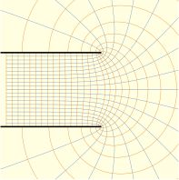
Figure 3.3.13 reproduces two field maps in the style of the plates of J. C. Maxwell's Treatise on Electricity and Magnetism (1873), in which equipotentials and field lines are drawn together. On the left is the region near the edge of a parallel-plate capacitor. Deep inside the capacitor the equipotentials are equally spaced parallel planes and the field is uniform (Problem 3.3.1). Near the edge they bulge out of the gap and the field lines "fringe" around the edges of the plates, always crossing the equipotentials at right angles. This exact picture was obtained with a conformal mapping, a two-dimensional technique beyond the scope of this course.

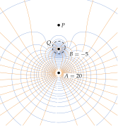
**Figure 3.3.13.** Equipotentials (blue) and field lines (orange) (a) at the edge of a parallel-plate capacitor (cross-section, with the plates as the two thick lines),

and (b) for two point charges of strengths 20 and -5 (arbitrary units), after Maxwell's Fig. II. P is the point of equilibrium, where \vec E=0 (AP=2AB). The dashed circle Q is the trace of the spherical surface of zero potential. — and (b) for two point charges of strengths $20$ and $- 5$ (arbitrary units), after Maxwell's Fig. II. $P$ is the point of equilibrium, where $E = 0$ ( $A P = 2 A B$ ). The dashed circle $Q$ is the trace of the spherical surface of zero potential.

On the right are two point charges of opposite sign and unequal magnitude, $q_{A} = 20$ and $q_{B} = - 5$ in arbitrary units, with $B$ at unit distance above $A$ . Two special features can be checked with the formulas of this section. Writing $r_{A}$ and $r_{B}$ for the distances from the two charges,

V \propto \frac{20}{r _{A}} - \frac{5}{r _{B}} .

The zero-potential surface $V = 0$ requires $r_{A} = 4 r_{B}$ . With $A$ at the origin and $B$ at $(0, 1)$ , $x^{2} + y^{2} = 16 [x^{2} + (y - 1)^{2}]$ , i.e. $x^{2} + (y - \frac{16}{15})^{2} = (\frac{4}{15})^{2}$ : a sphere of radius $4/15$ centred at $y = 16/15$ , enclosing the smaller charge (the dashed circle $Q$ ).
The point of equilibrium $P$ , where the two fields cancel, lies on the axis beyond $B$ : $20/ y^{2} = 5/ (y - 1)^{2}$ gives $2 (y - 1) = y$ , i.e. $y = 2$ , so $A P = 2 A B$ . A small positive charge placed at $P$ feels no force. The equipotential through $P$ crosses itself there, and the field lines that reach $P$ divide those that go to $B$ from those that escape to infinity.

Far away, the two charges look like a single charge $20 - 5 = 15$ , and the equipotentials become spheres.

Point charge and electric dipole

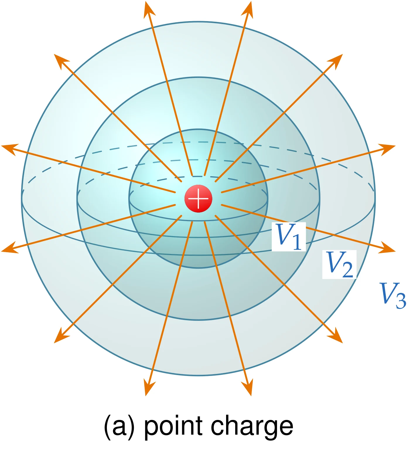
(b) Equipotentials (blue) r^2=C\cos\theta and field lines (orange) r=C\sin^2\theta of an ideal dipole whose moment points to the right (\theta measured from the dipole axis). The plane \theta=90^\circ is the surface V=0. — (b) Equipotentials (blue) $r^{2} = C cos θ$ and field lines (orange) $r = C sin^{2} θ$ of an ideal dipole whose moment points to the right ( $θ$ measured from the dipole axis). The plane $θ = 9 0^{\circ}$ is the surface $V = 0$ .

Point charge

For $V = q / (4 π ε_{0} r)$ the surfaces $V = const$ are the spheres $r = const$ centred on the charge, and the field lines are radial (Figure 3.3.14a). Equipotentials drawn for equal steps $Δ V$ are not equally spaced: from $d V / d r = - q / (4 π ε_{0} r^{2})$ , a step $Δ V$ corresponds to

Δ r ≃ \frac{4 π ε _{0} r ^{2}}{q} ∣Δ V ∣,

so the spacing grows like $r^{2}$ . Where the spheres spread apart the field $E = ∣ d V / d r ∣$ is small. In this way the picture shows the $1/ r^{2}$ decay of the Coulomb field.

Electric dipole

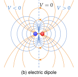
Two equal and opposite charges $\pm q$ a distance $d$ apart form an electric dipole of moment $p = q d$ , directed from $- q$ to $+ q$ . At distances $r ≫ d$ its potential is (Exercise 3.3.2)

V = \frac{p cos θ}{4 π ε _{0} r ^{2}},

where $θ$ is measured from the direction of $p$ (horizontal in Figure 3.3.14b). The equipotentials $V = const$ are therefore the surfaces

r^{2} = C cos θ, C = \frac{p}{4 π ε _{0} V},

with $V > 0$ on the side of the positive charge and $V < 0$ on the other, and the plane $θ = 9 0^{\circ}$ bisecting the dipole is the surface $V = 0$ . The field follows from the gradient in spherical coordinates,

E = - \frac{\partial V}{\partial r} a_{r} - \frac{1}{r} \frac{\partial V}{\partial θ} a_{θ} = \frac{p}{4 π ε _{0} r ^{3}} (2 cos θ a_{r} + sin θ a_{θ}) .

It falls off as $1/ r^{3}$ , one power faster than the field of a single charge, because seen from far away the two opposite charges almost cancel each other.

Every field line crosses every equipotential at a right angle, as the general argument requires. The dipole field reappears in Home exercise 3.3.5.

Drag the two charges of the dipole and watch the equipotentials (and the field lines crossing them at right angles) follow. Switch to a single charge to see the concentric spheres.

InteractiveLoading simulation…