Electromagnetic Fields and Waves: Notes, Solved Problems and Interactive Lab

Classification of media

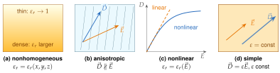
The relation $D = ε E$ looks simple, but $ε$ need not be a simple constant. Depending on how $ε_{r}$ behaves, media are classified as follows (Figure 3.4.3).

Nonhomogeneous medium. $ε_{r}$ is a function of the space coordinates, $ε_{r} = ε_{r} (x, y, z)$ . The atmosphere, whose density (and hence permittivity) decreases with height, is an example, and so is a capacitor insulated with layers of different materials (Exercises 3.4.3 and 3.4.4).
Anisotropic medium. $ε_{r}$ is a tensor. At a given point the response of the medium differs from direction to direction, and $D$ is in general not parallel to $E$ :

$D_{x} D_{y} D_{z} = ε_{0} ε_{xx} ε_{y x} ε_{z x} ε_{x y} ε_{y y} ε_{z y} ε_{x z} ε_{y z} ε_{z z} E_{x} E_{y} E_{z} .$

Many crystals and liquid crystals behave in this way.
Nonlinear medium. $ε_{r}$ depends on the field itself, $ε_{r} = ε_{r} (E)$ , so doubling $E$ does not double $D$ . The ferroelectric ceramics used in capacitors (Application 3.4.1) are strongly nonlinear.
Simple medium. A medium that is homogeneous, isotropic and linear is called a simple medium. Its permittivity is a single scalar constant.

The four kinds of media. (a) The permittivity changes from place to place. (b) The response depends on direction (here a layered crystal): \vec D and \vec E point in different directions. (c) D is not proportional to E: the response saturates at high fields. (d) A simple medium: \vec D is \varepsilon times \vec E, everywhere and in every direction. — **Figure 3.4.3.** The four kinds of media. (a) The permittivity changes from place to place. (b) The response depends on direction (here a layered crystal): $D$ and $E$ point in different directions. (c) $D$ is not proportional to $E$ : the response saturates at high fields. (d) A simple medium: $D$ is $ε$ times $E$ , everywhere and in every direction.

Unless stated otherwise we shall work with simple media, or with regions each of which is a simple medium, joined at boundaries. This covers a remarkably large part of engineering practice.

Typical values of the relative permittivity

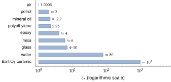
For most gases $ε_{r}$ is very close to 1: the Earth's atmosphere at sea level has $ε_{r} \approx 1.0006$ , which is why we may treat air as vacuum in almost every calculation. Liquids generally have relative permittivities between about 2 and 81. Petrol has $ε_{r} \approx 2$ , whereas water, whose molecules carry a large permanent dipole moment, has $ε_{r} \approx 81$ (about 80 at room temperature). For most solids $ε_{r}$ lies between 2 and 10. Mica and porcelain, for instance, have $ε_{r} \approx 6$ . Figure 3.4.4 shows the spread on a logarithmic scale.

Table 3.4.1. Approximate relative permittivities at low frequency and room conditions. Values depend on density, temperature, purity and frequency and should be read as typical.

Group	Material	$ε_{r}$	Typical use
Gases	air (sea level)	$1.0006$	everywhere (taken as 1)
Liquids	petrol, kerosene	$\approx 2$	fuels
	transformer (mineral) oil	$\approx 2.2$	transformer insulation
	water	$\approx 80$ – $81$	high-permittivity liquid
Solids	polypropylene	$\approx 2.2$	film capacitors
	polyethylene	$2.25$	cable insulation
	epoxy resin	$\approx 4$	cast insulation
	mica, porcelain	$\approx 6$	Worked example 3.4.1
	glass	$\approx 4$ – $10$	windows, display covers
	ceramics (BaTiO $_{3}$ -based)	$\sim 1 0^{3}$ (nonlinear)	multilayer capacitors

**Figure 3.4.4.** Typical relative permittivities (Table 3.4.1) on a logarithmic scale. Gases are practically vacuum, and most liquids and solids lie between 2 and 10. Water, with its strongly polar molecules, and ferroelectric ceramics stand far apart. (Glass is drawn at a mid-range value of 7.)

We must keep in mind that $ε_{r}$ varies with density, frequency and temperature. The values quoted refer to standard temperature and pressure and to static or low-frequency fields. The frequency dependence can be dramatic: the permanent dipoles of water follow a slowly varying field and give $ε_{r} \approx 80$ , but at optical frequencies they cannot follow at all, and the relative permittivity of water falls to $n^{2} \approx 1.3 3^{2} \approx 1.8$ .

Dielectrics and polarisation

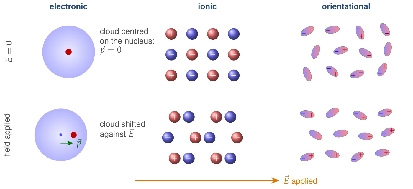
In some media the external field $E$ creates electric dipoles inside the material, or aligns dipoles that are already there. Such materials are called dielectrics, and the creation or alignment of these dipoles is called polarisation. Three microscopic mechanisms contribute (Figure 3.4.5):

electronic polarisation: the electron cloud of every atom is shifted slightly against the field, relative to the nucleus,
ionic polarisation: in an ionic crystal the positive and negative ions are displaced in opposite directions, and
orientational polarisation: molecules that carry a permanent dipole moment (water is the classic example) tend to turn into the direction of the field, against the disordering effect of thermal motion.

The three microscopic mechanisms of polarisation, without a field (top) and with a field pointing to the right (bottom). Electronic: the electron cloud is pulled against \vec E, the nucleus along it, and a small dipole \vec p appears. Ionic: positive ions shift along \vec E, negative ions against it (grey marks: the original positions). Orientational: permanent molecular dipoles, randomly oriented at \vec E=0, turn partly into the direction of the field. In all three cases the dipole moment points along \vec E. — **Figure 3.4.5.** The three microscopic mechanisms of polarisation, without a field (top) and with a field pointing to the right (bottom). Electronic: the electron cloud is pulled against $E$ , the nucleus along it, and a small dipole $p$ appears. Ionic: positive ions shift along $E$ , negative ions against it (grey marks: the original positions). Orientational: permanent molecular dipoles, randomly oriented at $E = 0$ , turn partly into the direction of the field. In all three cases the dipole moment points along $E$ .

Recall from Section 3.1 that two charges $+ Q$ and $- Q$ separated by the vector $d$ , drawn from the negative to the positive charge, form a dipole of moment $p = Q d$ [C·m]. We describe the dipoles of a material by their density.

Definition · Polarisation vector

The polarisation vector $P$ is the electric dipole moment per unit volume,

P = Δ v \to 0 lim \frac{\sum _{k} p _{k}}{Δ v} [C/ m^{2}],

the sum running over all dipoles in the small volume $Δ v$ .

The inner charges of Section 3.4.1 are the charges of these dipoles, and their density is

\overset{ρ}{ˉ} (E) with P = - \nabla \cdot P = ε_{0} χ E, (3.4.6)

as we shall show below. Comparing with Eq. (3.4.2), the vector $ε_{0} χ E$ introduced there is exactly the polarisation. In a linear dielectric the dipole density is proportional to the field, so $χ$ is a constant.

What is the sign of $χ$ ? Every mechanism listed above pushes the positive charges along $E$ and the negative charges against it. The vector drawn from the negative to the positive charge of each induced dipole therefore points along $E$ , and so does $P$ . Hence, in $P = ε_{0} χ E$ , the susceptibility is positive:

χ > 0, ε_{r} > 1, ε > ε_{0} .

Every material medium has a permittivity larger than that of vacuum.

In plain words

A dielectric is like a crowd that leans with the wind: each molecule gives a little in the direction of the field. The polarisation $P$ measures how much "leaning" there is per cubic metre.

The polarisation picture: bound charges

The polarisation picture. Left: without an external field the molecular dipoles of a dielectric (blue: -, red: +) point in random directions and \vec P=0. Right: a slab between two charged plates. The field aligns the dipoles. Inside the slab the + end of each dipole is next to the - end of its neighbour and the charges cancel, but on the two faces a net bound charge \mp\rho_{Sb} is left over, facing the free charge \pm\rho_S on the plates. — **Figure 3.4.6.** The polarisation picture. Left: without an external field the molecular dipoles of a dielectric (blue: $-$ , red: $+$ ) point in random directions and $P = 0$ . Right: a slab between two charged plates. The field aligns the dipoles. Inside the slab the $+$ end of each dipole is next to the $-$ end of its neighbour and the charges cancel, but on the two faces a net bound charge $\mp ρ_{S b}$ is left over, facing the free charge $\pm ρ_{S}$ on the plates.

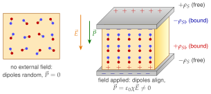
Figure 3.4.6 shows what polarisation looks like. Consider a uniformly polarised slab. Inside it, every small volume contains as many positive as negative dipole ends (the $+$ end of one dipole sits next to the $-$ end of the next), so the net charge density in the interior is zero. Only on the two faces is this cancellation incomplete: on the face where the dipoles point outwards a layer of positive dipole ends is left uncompensated, on the opposite face a layer of negative ends. These charges cannot leave the molecules they belong to. They are called bound (or polarisation) charges, to distinguish them from the free charges that we can move, add or remove, such as the charge on the plates. If $P$ is not uniform, the cancellation inside is incomplete too, and a bound volume charge appears.

The precise statement is short. A polarised dielectric acts, as far as its field is concerned, exactly like two charge distributions in vacuum:

Bound charges

ρ_{S b} ρ_{b} = P \cdot a_{n} [C/ m^{2}] on its surface, = \overset{ρ}{ˉ} = - \nabla \cdot P [C/ m^{3}] inside it, (3.4.7)

where $a_{n}$ is the outward normal of the dielectric. The derivation, which starts from the potential of a single dipole, is given in the box below. On a first reading you may take Eq. (3.4.7) as the mathematical form of the picture in Figure 3.4.6. Their sum is zero, as it must be for a body that was neutral: $\oint_{S} P \cdot d S - \int_{v} \nabla \cdot P d v = 0$ by the divergence theorem. In the slab of Figure 3.4.6 $P$ is uniform, $ρ_{b} = 0$ , and the bound charge sits only on the faces: $P$ points down, so $P \cdot a_{n} = + P$ on the lower face and $- P$ on the upper face.

With Eq. (3.4.7) we can now redo the bookkeeping of Section 3.4.1 in physical terms. Gauss's law for all charges,

\nabla \cdot (ε_{0} E) = ρ_{v} + ρ_{b} = ρ_{v} - \nabla \cdot P,

gives, after moving $\nabla \cdot P$ to the left,

\nabla \cdot (ε_{0} E + P) = ρ_{v} ⟹ D = ε_{0} E + P . (3.4.9)

This is the most general definition of $D$ . It holds even for nonlinear or anisotropic materials, and for materials that remain polarised without any field (electrets). In a linear, isotropic medium $P = ε_{0} χ E$ and we recover

D = ε_{0} E + P = ε_{0} (1 + χ) E = ε E . (3.4.10)

\vec D=\varepsilon_0\vec E+\vec P drawn with field lines, for a dielectric slab with \varepsilon_r=3 between two plates carrying \pm\rho_S (thin air gaps above and below the slab). Lines of \vec D start and end only on free charge: six lines everywhere. Lines of \varepsilon_0\vec E start and end on all charge: six in the air gaps, but four of them end on the bound charge of the slab, so only two cross the dielectric: the field inside is reduced by \varepsilon_r=3. Lines of \vec P exist only in the dielectric and run from the negative to the positive bound charge: four lines. Inside the slab, 6=2+4. — **Figure 3.4.7.** $D = ε_{0} E + P$ drawn with field lines, for a dielectric slab with $ε_{r} = 3$ between two plates carrying $\pm ρ_{S}$ (thin air gaps above and below the slab). Lines of $D$ start and end only on free charge: six lines everywhere. Lines of $ε_{0} E$ start and end on all charge: six in the air gaps, but four of them end on the bound charge of the slab, so only two cross the dielectric: the field inside is reduced by $ε_{r} = 3$ . Lines of $P$ exist only in the dielectric and run from the negative to the positive bound charge: four lines. Inside the slab, $6 = 2 + 4$ .

Physical picture

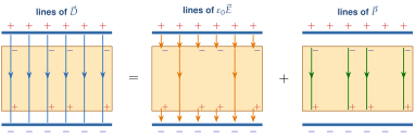
$D$ sees only the free charge $ρ_{v}$ , whereas $ε_{0} E$ sees all of it, free and bound. The bound charge always has the opposite sign to the free charge it faces, so it partly cancels it. In the slab of Figure 3.4.6 the plates carry $\pm ρ_{S}$ , so $D = ρ_{S}$ whatever the material, while $ε_{0} E = ρ_{S} - ρ_{S b}$ . With $E = D / ε = ρ_{S} / (ε_{r} ε_{0})$ this gives $ρ_{S b} = ρ_{S} (1 - 1/ ε_{r})$ : for the same free charge the field inside a dielectric is weaker by the factor $ε_{r}$ (Figure 3.4.7).

Quick check

A cube of dielectric is uniformly polarised, $P = P_{0} a_{z}$ . Where is the bound charge, and how much is there in total?

$ρ_{b} = - \nabla \cdot P = 0$ inside, because $P$ is constant. On the top face ( $a_{n} = a_{z}$ ) $ρ_{S b} = + P_{0}$ , on the bottom face ( $a_{n} = - a_{z}$ ) $ρ_{S b} = - P_{0}$ , on the four side faces $P \cdot a_{n} = 0$ . The total is zero.

Common mistake · Mixing free and bound charge

Writing $\oint_{S} D \cdot d S$ equal to the free plus the bound charge inside $S$ , or $\oint_{S} ε_{0} E \cdot d S$ equal to the free charge alone. Keep the two books apart: $D$ counts free charge only, $ε_{0} E$ counts all charge. Bound charge never appears in Gauss's law for $D$ , because it is already inside $ε$ .

3.4.3 Electrical properties of media

Classification of media

Typical values of the relative permittivity

Dielectrics and polarisation

The polarisation picture: bound charges