Electromagnetic Fields and Waves: Notes, Solved Problems and Interactive Lab

Consider a scalar function $f (x, y, z)$ . Its gradient $\nabla f$ is a vector field, and we may take the divergence of that vector field. The result is a scalar again, called the Laplacian of $f$ :

Laplacian in Cartesian coordinates

\nabla \cdot (\nabla f) = Δ f = \nabla^{2} f = \frac{\partial ^{2} f}{\partial x ^{2}} + \frac{\partial ^{2} f}{\partial y ^{2}} + \frac{\partial ^{2} f}{\partial z ^{2}} . (2.2.10)

The derivation is a single line: the components of $\nabla f$ are $\partial f / \partial x$ , $\partial f / \partial y$ , $\partial f / \partial z$ , and (2.2.6) differentiates each once more with respect to its own coordinate. The notations $Δ f$ and $\nabla^{2} f$ are both in common use, and we shall mostly write $\nabla^{2} f$ , which reminds us of $\nabla \cdot \nabla f$ .

Meaning: a comparison with the neighbours

Start in one dimension, where the Laplacian is just the second derivative $f^{''} (x)$ . Take a point $x$ and its two neighbours $x \pm h$ . A Taylor expansion gives $f (x \pm h) = f (x) \pm h f^{'} (x) + \frac{1}{2} h^{2} f^{''} (x) \pm \dots$ , and the average of the two neighbours is

\frac{f ( x + h ) + f ( x - h )}{2} = f (x) + \frac{h ^{2}}{2} f^{''} (x) + \dots

(the first-derivative terms cancel). So $f^{''} > 0$ means that $f (x)$ lies below the average of its neighbours (the bottom of a valley), $f^{''} < 0$ that it lies above it (the top of a crest), and $f^{''} = 0$ that it equals the average (a straight line), as Figure 2.2.9 shows. In two dimensions the same expansion with the four neighbours $(x \pm h, y)$ , $(x, y \pm h)$ gives $average = f + \frac{h ^{2}}{4} \nabla^{2} f + \dots$ , and in three dimensions, with the six neighbours, $average = f + \frac{h ^{2}}{6} \nabla^{2} f + \dots$

The Laplacian as “value minus average of the neighbours”. In (a) to (c) the black dots are the neighbours f(x\pm h), the green circle is their average (the midpoint of the dashed chord) and the red dot is f(x). The three curves are 0.35x^2+0.6, 0.3x+1 and -0.35x^2+1.4. The gap between the red dot and the green circle is \tfrac12h^2f'' (to leading order). (d) In a plane the average is taken over four neighbours (six in space). Where \nabla^2f=0, the value at \mathrm P equals that average up to small terms of order h^4. — **Figure 2.2.9.** The Laplacian as “value minus average of the neighbours”. In (a) to (c) the black dots are the neighbours $f (x \pm h)$ , the green circle is their average (the midpoint of the dashed chord) and the red dot is $f (x)$ . The three curves are $0.35 x^{2} + 0.6$ , $0.3 x + 1$ and $- 0.35 x^{2} + 1.4$ . The gap between the red dot and the green circle is $\frac{1}{2} h^{2} f^{''}$ (to leading order). (d) In a plane the average is taken over four neighbours (six in space). Where $\nabla^{2} f = 0$ , the value at $P$ equals that average up to small terms of order $h^{4}$ .

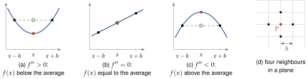
The same comparison holds for a smooth average over a small sphere. If we average $f$ over the surface of a sphere of radius $a$ centred at $P$ ,

\overset{ˉ}{f} = f (P) + \frac{a ^{2}}{6} \nabla^{2} f_{P} + \dots (2.2.11)

(the derivation is in the box below). So $\nabla^{2} f > 0$ means that $f$ at $P$ is lower than the average of its surroundings, $\nabla^{2} f < 0$ means that it is higher, and $\nabla^{2} f = 0$ means that $f$ at every point equals the average of its neighbourhood. Such a function (unless it is constant) can have no local maximum or minimum inside the region: a maximum would have to be higher than its own average. Equations of the form $\nabla^{2} V = 0$ (Laplace's equation) and $\nabla^{2} V = - ρ_{v} / ε_{0}$ (Poisson's equation) govern the electrostatic potential (Section 3.3).

In plain words

The Laplacian measures how much a function at a point differs from the average of its immediate surroundings: positive in a "dip", negative on a "bump", zero where the point is exactly the average of its neighbours. It is the divergence of the gradient: a dip is a place where the uphill arrows all point away from it.

Quick check

Compute $\nabla^{2} f$ for $f = x^{2} + y^{2} + z^{2}$ and for $f = x^{2} - y^{2}$ . What do the results say about the point $(0, 0, 0)$ ?

$\nabla^{2} (x^{2} + y^{2} + z^{2}) = 2 + 2 + 2 = 6 > 0$ : the origin is a minimum, lower than the average around it. $\nabla^{2} (x^{2} - y^{2}) = 2 - 2 = 0$ : the origin is a saddle (up along $x$ , down along $y$ ), and $f (0) = 0$ is exactly the average of its surroundings, so it is neither a maximum nor a minimum.

A few useful identities

For a vector field, the Laplacian in Cartesian coordinates acts on each component: $\nabla^{2} A = \nabla^{2} A_{x} a_{x} + \nabla^{2} A_{y} a_{y} + \nabla^{2} A_{z} a_{z}$ . It is linked to curl and divergence by $\nabla \times (\nabla \times A) = \nabla (\nabla \cdot A) - \nabla^{2} A$ . The "product rules" of the operators, all of which can be checked component by component, are

\nabla (f g) \nabla \cdot (f A) \nabla \times (f A) = f \nabla g + g \nabla f, = f \nabla \cdot A + A \cdot \nabla f, = f \nabla \times A + \nabla f \times A,

\nabla \cdot (A \times B) = B \cdot (\nabla \times A) - A \cdot (\nabla \times B) .

2.2.6 The Laplacian

Meaning: a comparison with the neighbours