Section 2.3 · Topic 10 of 11
2.3.10 Differential operators in curvilinear coordinates
In Section 2.2 the gradient, divergence, curl and Laplacian were defined and computed in Cartesian coordinates, where the nabla operator is simply . Most fields of electromagnetics, however, are much simpler in cylindrical or spherical coordinates: the field of a point charge is , that of a line charge . Converting such fields to Cartesian form only to differentiate them would be slow and would hide their simple structure. We therefore want the four operators directly in curvilinear coordinates.
It is tempting to write "" in spherical coordinates, but this is wrong for two reasons.
- Angles are not lengths. A derivative with respect to an angle is a change per radian, not a change per metre (Figure 2.3.28). The scale factors found in Section 2.3.6 must enter.
- The unit vectors move. Even when the missing scale factors are put in, the unit vectors are themselves functions of position, see Eq. (2.3.38), so the divergence and the curl can no longer be obtained by simply "dotting" or "crossing" the operator with the components of the field, as was done in Cartesian coordinates.
The reliable way is to go back to the meaning of each operator, which does not refer to any coordinate system:
- the gradient gives the change of a scalar along a displacement, ,
- the divergence is the net outward flux per unit volume of a vanishingly small volume, and
- the curl is the circulation per unit area around a vanishingly small loop.
We now apply these definitions to the small curvilinear volume and surface elements of a general orthogonal system with scale factors . All results are valid for any orthogonal coordinate system. Cartesian, cylindrical and spherical coordinates are then obtained by inserting their scale factors from Table 2.3.4.
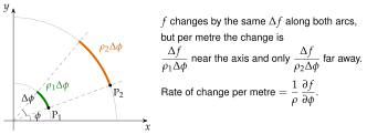
Writing , or computing a spherical divergence as . A unit check already exposes the error: has the units of , not of per metre.
Gradient
Recall the Cartesian form from Section 2.2,
and its key property: for a small displacement ,
The relation involves only the scalar change and the geometric displacement , so it holds in every coordinate system and can serve as the definition of the gradient. We use it in three steps.
Let . By the chain rule,
Write the unknown gradient as . With from Eq. (2.3.42) and the orthonormality of the unit vectors ( for , for ),
These two expressions must agree for arbitrary , so the coefficients must agree: , i.e. .
The meaning of the factors is plain: is the change of per radian, but a gradient component must be a change per metre. At distance from the axis one radian of is metres of arc, so we divide by (Figure 2.3.28). Every component of the gradient therefore has the units of per metre (e.g. V/m when is a potential in volts).
Each component of the gradient is "how fast changes per metre when you walk along that coordinate direction". Differentiate with respect to the coordinate, then divide by the number of metres that one unit of the coordinate represents ().
For only the radial derivative survives in Eq. (2.3.50): . This is the result obtained with considerably more effort in Cartesian form in Section 2.2 (gradient of with the source at the origin). Choosing the coordinate system that matches the symmetry of the problem is half of the solution. This lesson will be repeated many times in Sections 3.1 to 3.3.
Compute the gradient of with Eq. (2.3.50). Why is the answer not a surprise?
, which by Eq. (2.3.46) is exactly . No surprise: , and .
Divergence
The divergence of at a point is the net outward flux of per unit volume, in the limit of a vanishingly small volume around the point:
In Cartesian coordinates, a small box has opposite faces of equal area, and only the change of the field component across the box matters. In curvilinear coordinates there is a new effect: the opposite faces of a small box need not have the same area. Let us see this first in the most important case, and then in general.
The radial faces of a spherical box
Take the small spherical brick of Figure 2.3.23, between and , and , and , and look only at its two faces on which is constant. On them only the radial component crosses the surface.
- Outer face (at , outward normal ): its area is , so its outward flux is .
- Inner face (at , outward normal ): its area is , so its outward flux is .
The outer face is larger than the inner one, so what counts is not the change of alone but the change of the product (field times area factor). To first order in the net outward flux through the two faces is
and dividing by the volume gives the radial part of the spherical divergence,
The other two pairs of faces work in the same way. The faces have area , which depends on through , and this produces . The faces have area , which does not depend on , so they produce simply .
Any orthogonal system
The same bookkeeping in a general orthogonal system gives the general formula below, with the details in the box. The result says: for each pair of faces, differentiate "component area factor of that face", then divide by the volume factor .
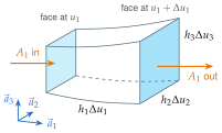
Take as the small curvilinear box of Figure 2.3.29(a), bounded by the coordinate surfaces and , and , and . Its edges are , , and its volume is .
Consider first the pair of faces on which is constant. On the face at the outward normal is , the face has area , and only the component crosses it. Its outward flux is
On the opposite face at the outward normal is , so its outward flux is . The crucial point is that the scale factors and may themselves depend on : the two faces need not have the same area. In spherical coordinates, for example, the face at is larger than the face at by the factor . Therefore it is the product (the flux per unit ) whose change we must compute. To first order in ,
The other two pairs of faces give, in exactly the same way,
and
Adding the three contributions and dividing by , the products of increments cancel and, in the limit, the approximation becomes exact. This is Eq. (2.3.52).
For Cartesian coordinates () Eq. (2.3.52) reduces to the familiar of Section 2.2. For cylindrical coordinates, and
which is Eq. (2.3.53) because does not depend on . For spherical coordinates, and
taking out of each derivative the factors that do not depend on the variable of differentiation gives Eq. (2.3.54), in agreement with the direct argument above.
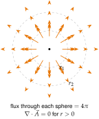
The factor in front of has a direct physical meaning. Consider the purely radial field , whose magnitude falls off exactly as the area of a sphere grows (Figure 2.3.30(a)). Its flux through any sphere centred at the origin is , the same for every radius: whatever enters a spherical shell through its inner face also flows out through its outer face. Accordingly Eq. (2.3.54) gives for every , even though the field certainly decreases with . A naive "" would have given the wrong value . The only place where the flux can originate is the origin itself, where the field is not defined. This is precisely the situation of a point charge, and it will be the heart of Gauss's law in Section 3.2. By contrast, for the position vector we find , which agrees with the Cartesian value .
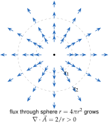
Compute (i) in spherical coordinates and (ii) and in cylindrical coordinates.
(i) . (ii) and for . The field (the shape of the field of a line charge) plays for cylinders the role that plays for spheres.
The explorer below draws the field in a plane . Move the probe box around: wherever the box stays away from the axis, the flux entering it equals the flux leaving it and the divergence is zero, and only a box that encloses the axis shows a net outward flux.
Differentiating only the component: writing instead of , or instead of . Multiply by the area factor first, then differentiate, then divide.
Curl
The component of the curl along a unit vector is the circulation of per unit area around a vanishingly small loop that bounds an area with normal , the loop being traversed in the right-hand sense with respect to :
As for the divergence, there is one new effect compared with Cartesian coordinates: opposite sides of a small curvilinear loop need not have the same length.
The z component of the curl in cylindrical coordinates
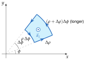
Take the small loop of Figure 2.3.31 in a plane , bounded by the circles and and the half-planes and , traversed counter-clockwise seen from (so that its normal is ). Along each side only one component of contributes to :
- The two straight sides (length ) contribute at (travelled outwards) and at (travelled inwards). Together, to first order, they give .
- The two arcs contribute (outer arc, travelled forwards) and (inner arc, travelled backwards). The outer arc is longer, so it is the product that matters. Together the arcs give .
Dividing the circulation by the area gives
Any orthogonal system
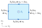
In general, the component of the curl comes from a small loop on a surface (Figure 2.3.29(b)), whose sides have lengths and . Exactly as above, the circulation involves the changes of the products and , and the area is . The box gives the details.
For the component take the small loop on a surface shown in Figure 2.3.29(b): its sides run along (length ) and along (length ), and its area is . Going round the loop as indicated (first along , then along , so that the normal is ), the four sides contribute
since along a side on which only changes, , and the top and left sides are traversed backwards. Grouping right with left and bottom with top, to first order,
Dividing by gives the component, and the other two follow by cyclic permutation :
Exactly as the Cartesian curl of Section 2.2, these three lines can be packed into a determinant: expanding the determinant of Eq. (2.3.57) along its first row and dividing by reproduces Eq. (2.3.56) term by term (e.g. the term is ). For cylindrical coordinates with the third line is the result found directly from Figure 2.3.31.
In the determinants the derivatives act only on the third row, and the coordinates must be listed in their right-handed order. Written out component by component, the cylindrical curl is
and the spherical curl is
The curl formulas look long, but each bracket is the same recipe as for the divergence, applied to a loop instead of a box: multiply each component by the length factor of its side (), take the "crossed" derivatives, and divide by the area of the loop.
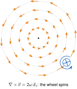
Two quick applications show what the curl measures (Figure 2.3.32). (i) A purely radial field that depends only on , , has and , so every bracket of Eq. (2.3.61) vanishes: . Such a field has no circulation at all, and the field of a point charge will be of this kind.
(ii) The velocity field of a body rotating rigidly about the axis with angular velocity is . By Eq. (2.3.60), : a uniform curl, parallel to the axis of rotation, equal to twice the angular velocity. A small paddle wheel placed anywhere in this flow turns, as the picture of Section 2.2 suggests. On the other hand, the field , which also "goes round", has for : circulating field lines do not by themselves imply a non-zero curl.
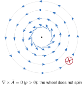
The field has constant magnitude and circles the axis. Is it curl-free?
No: . Only the special decrease makes a circulating field curl-free, see Figure 2.3.32(b).
Laplacian
The Laplacian of a scalar function is the divergence of its gradient, . In Cartesian coordinates this is the sum of the three second derivatives. In a general orthogonal system we simply insert the components of the gradient, Eq. (2.3.48), as into the divergence, Eq. (2.3.52):
For the spherical case, and the three ratios in Eq. (2.3.62) are , and . Dividing each term by and moving constant factors out of the derivatives yields Eq. (2.3.64). The cylindrical form follows in the same way with and the ratios , , .
Two simple but important checks:
Functions whose Laplacian vanishes are called harmonic, and these two will reappear as the potentials of a point charge and of a line charge (Section 3.3).
Compute in spherical coordinates and check the result in Cartesian coordinates.
. In Cartesian form and .
The formulas above are for the Laplacian of a scalar. The Laplacian of a vector field is defined through . Only in Cartesian coordinates does it reduce to the Laplacian of each component, . In cylindrical and spherical coordinates is not the -component of , again because the unit vectors vary with position.
All four operators on one page
Every formula of this section is one and the same general expression with filled in. The following box is the page to keep beside you for the rest of the course.
Gradient (scalar vector):
Divergence (vector scalar):
Curl (vector vector):
Laplacian (scalar scalar), , i.e. the first two formulas one after the other:
| scale factors | Cartesian | cylindrical | spherical |
|---|---|---|---|
- Write the field in the system that matches its symmetry and read off or (in the right-handed order of the coordinates).
- Take from the table and form the products that the formula asks for (, , …) before differentiating.
- Differentiate with respect to one coordinate at a time, holding the other two fixed.
- Divide by the indicated scale-factor products and simplify.
- Check: units (each adds "per metre"), and a special case you know (e.g. , , ).