Electromagnetic Fields and Waves: Notes, Solved Problems and Interactive Lab

In Cartesian coordinates $(u_{1}, u_{2}, u_{3}) = (x, y, z)$ , each ranging over $(- \infty, \infty)$ . The coordinate surfaces $x = const$ , $y = const$ , $z = const$ are planes parallel to the coordinate planes, and a point $P (x, y, z)$ is their intersection (Figure 2.3.4).

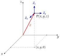
A point \mathrm P(x,y,z) in Cartesian coordinates, its position vector \vec r, and the unit vectors at \mathrm P. The Cartesian unit vectors are the same at every point. — **Figure 2.3.4.** A point $P (x, y, z)$ in Cartesian coordinates, its position vector $r$ , and the unit vectors at $P$ . The Cartesian unit vectors are the same at every point.

The position vector is $r = x a_{x} + y a_{y} + z a_{z}$ , so

\frac{\partial r}{\partial x} \frac{\partial r}{\partial y} \frac{\partial r}{\partial z} = a_{x}, h_{x} = 1, = a_{y}, h_{y} = 1, = a_{z}, h_{z} = 1. (2.3.9)

All scale factors are one (the coordinates themselves are lengths), and Eqs. (2.3.6), (2.3.7), (2.3.8) become (Figure 2.3.5)

Differential elements in Cartesian coordinates

d ℓ = d x a_{x} + d y a_{y} + d z a_{z}, (2.3.10)

d S_{x} d S_{y} d S_{z} = a_{x} d y d z, = a_{y} d z d x, = a_{z} d x d y, (2.3.11)

d V = d x d y d z . (2.3.12)

The unit vectors $a_{x}, a_{y}, a_{z}$ do not depend on position, which is what makes Cartesian coordinates so simple: they can be taken outside every derivative and every integral.

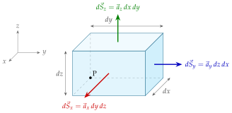
The differential volume dV=dx\,dy\,dz in Cartesian coordinates and its three visible faces as oriented areas. Each face lies on a coordinate plane (x, y or z constant), its normal is the corresponding unit vector, and its area is the product of the two edges that lie in it. — **Figure 2.3.5.** The differential volume $d V = d x d y d z$ in Cartesian coordinates and its three visible faces as oriented areas. Each face lies on a coordinate plane ( $x$ , $y$ or $z$ constant), its normal is the corresponding unit vector, and its area is the product of the two edges that lie in it.

Move the point in the explorer below and watch the three coordinate planes $x$ , $y$ , $z = const$ that meet at it, while the unit vectors $a_{x}$ , $a_{y}$ , $a_{z}$ stay the same at every point.

InteractiveLoading simulation…

Areas and volumes as integrals

The area of a surface is the sum of the areas of the small patches that make it up, $S = \int_{S} d S$ , and the volume of a region is $V = \int_{V} d V$ . The next two examples apply this with the Cartesian elements. The same idea, with the cylindrical elements, is used in Examples 2.3.12 to 2.3.14.

Example 2.3.4Area of a rectangle Example 2.3.5Volume of a rectangular box

Line integrals

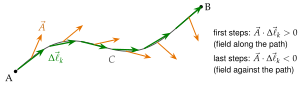
Let $C$ be a path from a point $A$ to a point $B$ and $A$ a vector field. Divide $C$ into small steps $Δ ℓ_{k}$ , each pointing along the path in the direction of travel. At each step form the dot product $A \cdot Δ ℓ_{k}$ (the tangential component of the field times the step length), add, and let the steps become infinitesimal (Figure 2.3.6):

\int_{C} A \cdot d ℓ = Δ ℓ_{k} \to 0 lim k \sum A \cdot Δ ℓ_{k} . (2.3.13)

The result is a scalar. If $A$ is a force it is the work done along the path, and if $A$ is an electric field, $- \int_{C} E \cdot d ℓ$ will be the potential difference (Section 3.3). When $C$ is closed, the integral is written $\oint_{C}$ and called the circulation (Section 2.2.4).

The line integral as a sum. The path C from \mathrm A to \mathrm B is divided into small steps \Delta\vec\ell_k (green) in the direction of travel, and at each step the field \vec A (orange) is projected onto the step. Steps on which the field helps contribute positively, steps on which it opposes contribute negatively, and steps across the field contribute nothing. — **Figure 2.3.6.** The line integral as a sum. The path $C$ from $A$ to $B$ is divided into small steps $Δ ℓ_{k}$ (green) in the direction of travel, and at each step the field $A$ (orange) is projected onto the step. Steps on which the field helps contribute positively, steps on which it opposes contribute negatively, and steps across the field contribute nothing.

How to evaluate it

In Cartesian coordinates, by Eq. (2.3.10),

A \cdot d ℓ = A_{x} d x + A_{y} d y + A_{z} d z .

On the path, the coordinates are not independent: we use the equations of the path to express everything in terms of a single variable, and that variable's start and end values are the limits. Along a straight line parallel to an axis only one differential survives (e.g. $d x = d z = 0$ along a line parallel to $y$ ). The direction of travel is taken care of by the limits alone: we always write $d ℓ = d x a_{x} + d y a_{y} + d z a_{z}$ with plus signs, and a path travelled towards decreasing $y$ simply has a lower limit larger than the upper one.

Recipe · Evaluating a line integral

\int_{C} A \cdot d ℓ

Describe the path: the equations that hold along it, its start point and its end point.
Write $A \cdot d ℓ = A_{x} d x + A_{y} d y + A_{z} d z$ (always with plus signs).
Use the path equations to remove all but one variable (differentials of fixed coordinates are zero).
Integrate from the start value of that variable (lower limit) to its end value (upper limit), even if the lower limit is the larger number.

Common mistake

Counting the direction of travel twice. For a path that runs from $y = 3$ down to $y = 1$ , writing $d ℓ = - d y a_{y}$ and integrating from $3$ to $1$ reverses the sign twice and gives the wrong answer. Either keep $d ℓ = d y a_{y}$ and the limits $3 \to 1$ (the method of this book), or use $d ℓ = ∣ d y ∣$ with limits $1 \to 3$ and the tangent $- a_{y}$ , but never both.

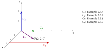
The four examples below use the paths of Figure 2.3.7.

The four integration paths of the line-integral examples. C_1: from (3,0,0) to (3,4,0), parallel to the y-axis. C_2: along the z-axis from the origin to (0,0,2). C_3: along the y-axis from y=3 *down* to y=1. C_4: along the line y=x in the xy-plane from \mathrm O to \mathrm P(2,2,0). The arrows give the direction of travel. — **Figure 2.3.7.** The four integration paths of the line-integral examples. $C_{1}$ : from $(3, 0, 0)$ to $(3, 4, 0)$ , parallel to the $y$ -axis. $C_{2}$ : along the $z$ -axis from the origin to $(0, 0, 2)$ . $C_{3}$ : along the $y$ -axis from $y = 3$ *down* to $y = 1$ . $C_{4}$ : along the line $y = x$ in the $x y$ -plane from $O$ to $P (2, 2, 0)$ . The arrows give the direction of travel.

Example 2.3.6Line integral along a line parallel to the

y

-axis Example 2.3.7Line integral along the

z

-axis Example 2.3.8Direction of travel Example 2.3.9Line integral along an oblique line

Surface integrals and flux

The flux of a vector field through an open surface $S$ is obtained in the same way as a line integral: divide $S$ into small patches $Δ S_{k} = a_{n} Δ S_{k}$ , take the normal component of the field on each (Figure 2.2.5), add, and refine:

Ψ = \int_{S} A \cdot d S = Δ S_{k} \to 0 lim k \sum A \cdot a_{n} Δ S_{k} . (2.3.14)

An open surface has two sides, and the choice of $a_{n}$ (the orientation) must be stated, because reversing it changes the sign of the flux. (For a closed surface the outward normal is the standard choice, as in the definition of divergence.) On the planes $x = const$ , $y = const$ , $z = const$ the oriented area elements are those of Eq. (2.3.11), possibly with a minus sign if the opposite orientation is chosen.

Recipe · Evaluating a flux integral

\int_{S} A \cdot d S

Identify the surface (which coordinate is constant on it, and the ranges of the other two) and its orientation $a_{n}$ .
Write $d S = a_{n} d S$ with the area element of that coordinate surface, e.g. $d S = a_{x} d y d z$ on $x = const$ .
Keep only the normal component $A \cdot a_{n}$ , and insert the constant coordinate of the surface.
Integrate over the two remaining coordinates between the limits that describe the surface.

Example 2.3.10Flux through a rectangle in the

y z

-plane

2.3.3 Cartesian coordinates

Areas and volumes as integrals

Line integrals

How to evaluate it

Surface integrals and flux

In this part

Examples · 7