Section 2.3 · Topic 6 of 11
2.3.6 Spherical coordinates
Cartesian coordinates are perfect for boxes and planes, and the cylindrical coordinates of Section 2.3.4 are perfect for wires and pipes. Many of the most important problems of electromagnetics, however, are organised around a single point: the field of a point charge, of a charged sphere, of a small antenna seen from far away. In such problems the natural questions are "how far from the centre?" and "in which direction?". Spherical coordinates answer exactly these two questions.
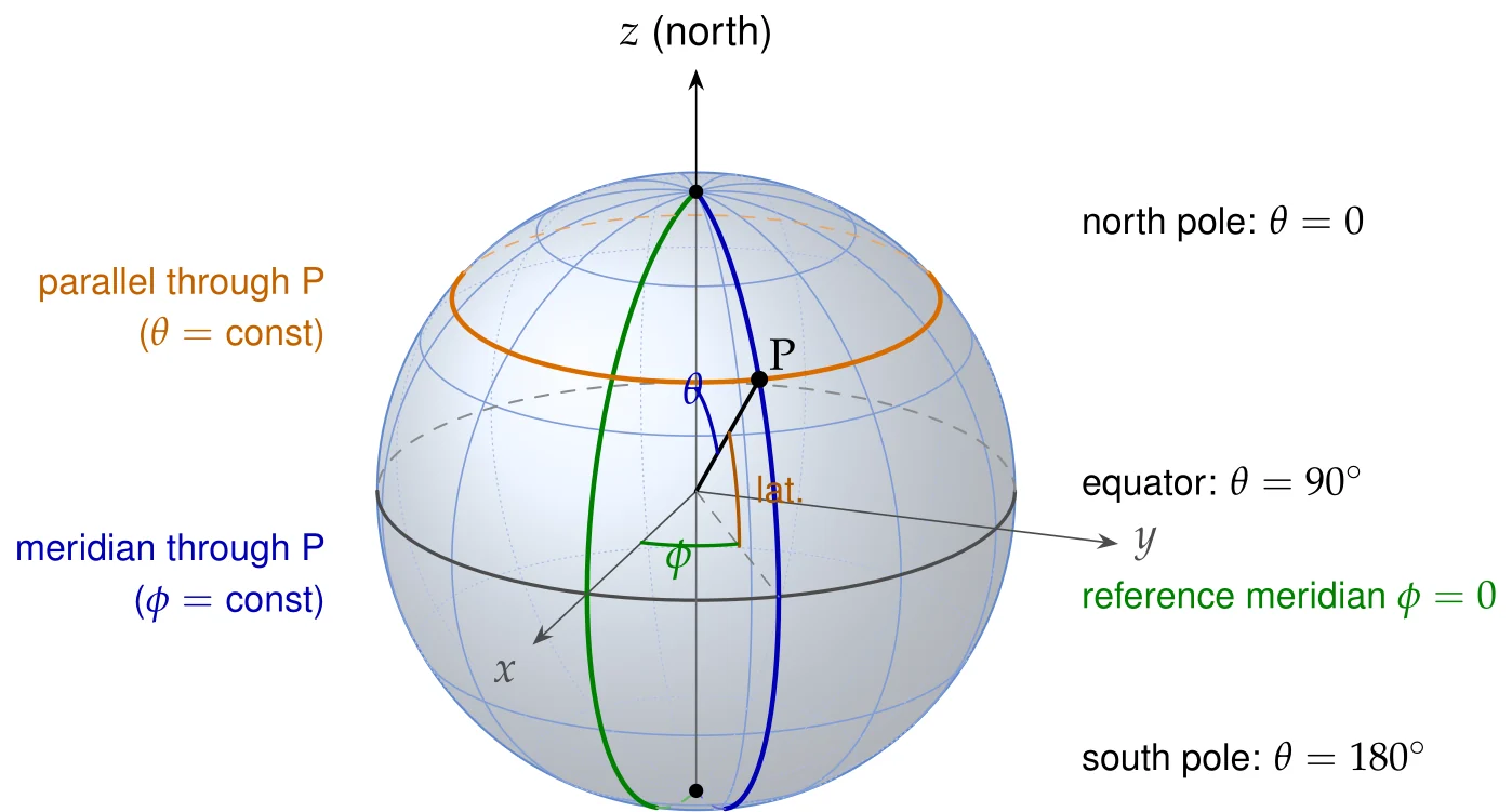
You already use spherical coordinates whenever you look at a map. A place on the Earth is given by two angles, its latitude (how far north or south of the equator) and its longitude (how far east or west of a reference meridian). Together with the distance from the centre of the Earth, these two angles fix the point completely. Spherical coordinates are the same idea, with two small changes of convention that we explain below (Figure 2.3.16).
We build the spherical system in the same way as the cylindrical one: coordinates, position vector, unit vectors and scale factors, and differential elements. We then compare the three systems of the course, learn to convert vector components between them, and finally use the new elements to compute areas, volumes and fluxes over spheres.
Definition of the coordinates
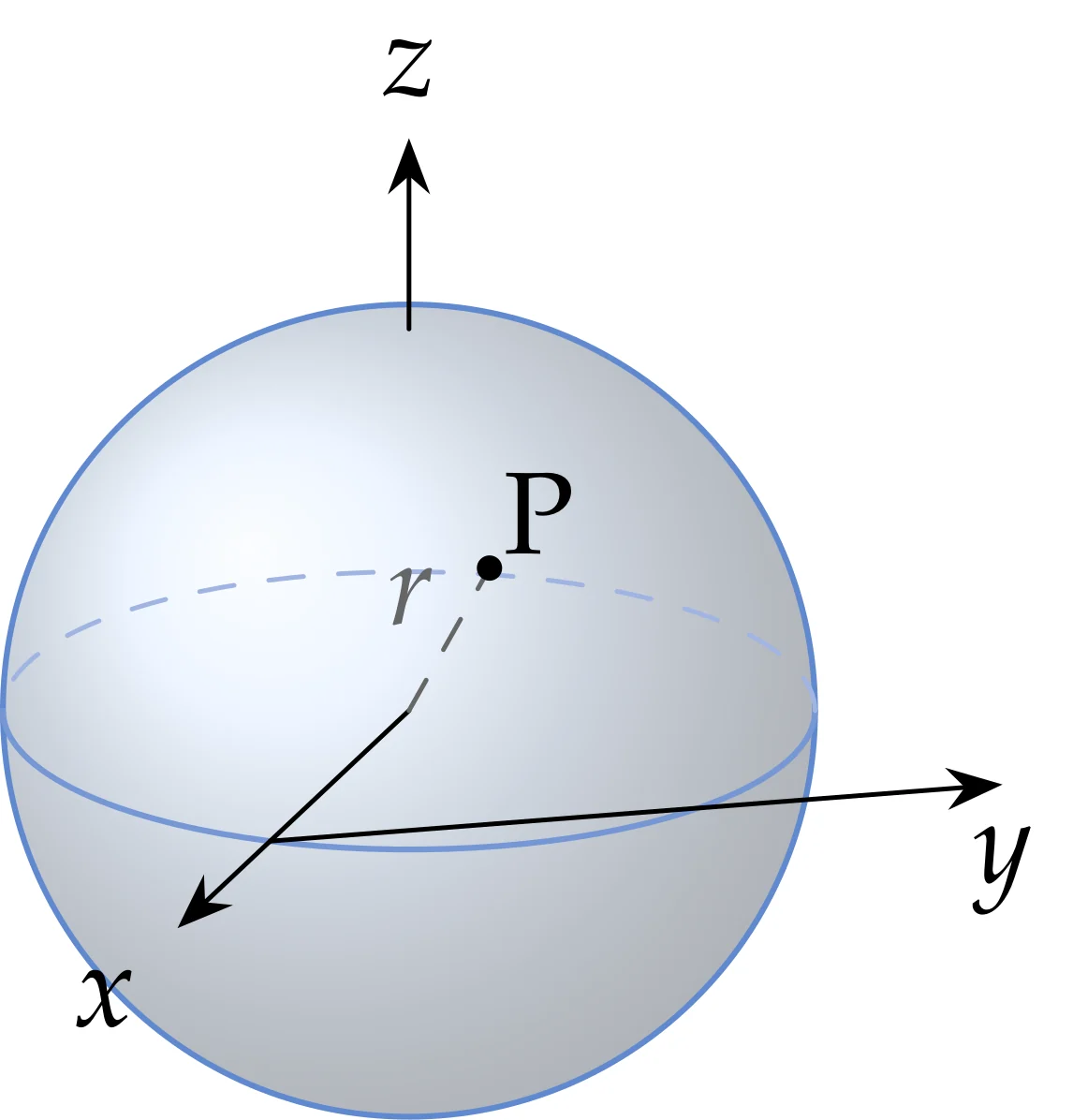
A point in space is located by three numbers , see Figure 2.3.18(a):
- the radial distance is the distance from the origin O to P, ,
- the polar angle (zenith angle) is the angle between the positive axis and the line OP, , and
- the azimuthal angle is the angle, measured in the -plane from the positive axis towards the positive axis, between the axis and the projection of OP onto the -plane, . It is the same angle as in cylindrical coordinates.
Note the ranges carefully: sweeps a full turn, but only runs from the "north pole" () to the "south pole" (). This is enough: once we know how far down from the north pole the point is () and on which side of the axis it lies (), every direction has been reached exactly once.
The geographic picture
Figure 2.3.16 makes the analogy with the globe precise. Geographers measure the latitude from the equator (from S to N), whereas we measure from the north pole, from to , so for points in the northern hemisphere and in the southern one. Geographers measure the longitude from to east or west, while we measure eastwards only, from to (in radians ). A circle of latitude (a parallel) is a curve on which is constant, and a meridian is a half circle from pole to pole on which is constant. We shall use the words "parallel" and "meridian" in exactly this sense.
Letting run from to . Every point would then be covered twice (once with and once "from the other side" with ), and surface and volume integrals come out wrong: since for , the second half cancels the first (for example would give a sphere zero area), and with everything would be counted twice. The correct ranges are and .
Coordinate surfaces
Each coordinate, held constant, defines a coordinate surface (Figures 2.3.17 and 2.3.18(b)):
- is a sphere centred at the origin,
- is a circular cone with its apex at the origin and the axis as its axis (for the cone opens up into the -plane, and for it opens downwards), and
- is a half-plane hinged on the axis.
The point P is the single common point of one sphere, one cone and one half-plane. These three surfaces meet at right angles to each other at every point, which is why the spherical system, like the Cartesian and the cylindrical ones, is an orthogonal coordinate system. The intersection of two coordinate surfaces is a coordinate curve: the sphere and the cone meet in a parallel (along which only varies), the sphere and the half-plane in a meridian (only varies), and the cone and the half-plane in a ray from the origin (only varies).

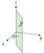
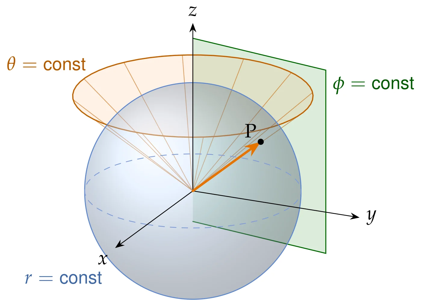
Drag , and and watch the sphere, the cone and the half-plane through P move, and see how the three unit vectors , , turn with the point while staying mutually perpendicular.
Which surfaces are described by (i) , (ii) , (iii) , (iv) , (v) ?
(i) The -plane (the "cone" has opened up flat). (ii) A cone with half-angle opening upwards around the axis. (iii) A cone with half-angle opening downwards around the axis. (iv) The half-plane , (the right half of the -plane). (v) The sphere of radius centred at the origin.
Position vector and the relations with Cartesian coordinates
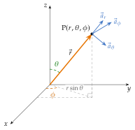
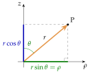
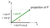
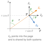
To relate to we project the position vector of P (length ) twice, as shown in Figure 2.3.19.
- In the vertical half-plane that contains P (panel a), the projection of onto the axis is , and its projection onto the -plane has length . This horizontal length is precisely the cylindrical radial distance of Section 2.3.4.
- In the -plane (panel b), the horizontal projection of length makes the angle with the axis, so it splits into along and along .
Hence
and the position vector of P reads
Inverting Eq. (2.3.30),
The first relation is Pythagoras' theorem in three dimensions. The arccos function returns values in , which is exactly the range of , so the polar angle is uniquely fixed by . For the azimuth this is not so: alone cannot distinguish from , and alone cannot distinguish from . The azimuth is the angle whose cosine and sine are given by Eq. (2.3.32). Equivalently, with the quadrant chosen according to the signs of and . Since , these are the same relations as for the cylindrical . On the axis () the azimuth is undefined, just as is undefined at the origin. Such exceptional points are harmless in integrals.
Computing the azimuth as with a calculator and stopping there. The calculator returns an angle between and , which is wrong whenever . Always look at the signs of and to decide the quadrant (or use the two-argument function atan2(y,x)).
Find the spherical coordinates of the point .
and . Then , so and , i.e. (, second quadrant). The calculator value points into the wrong quadrant.
The magnitude of is the coordinate , which is why the same letter is used. Do not confuse the spherical (distance from the origin) with the cylindrical (distance from the axis): , and the two coincide only in the -plane.
Unit vectors and scale factors
In Section 2.3.2 we learnt the recipe that produces the unit vectors and the scale factors of any orthogonal coordinate system : differentiate the position vector with respect to one coordinate while keeping the other two fixed,
The vector is tangent to the curve traced out by P when only changes. Its direction is the unit vector , and its length tells us how many metres P moves per unit change of . Let us apply the recipe to Eq. (2.3.31), one coordinate at a time.
Radial direction
Only changes, so we differentiate Eq. (2.3.31) with and held fixed:
Increasing moves P straight away from the origin, one metre per metre: .
Polar direction
Only changes:
Increasing moves P "southwards" along a meridian, a circle of radius , so a change (in radians) is an arc of length , hence .
Azimuthal direction
Only changes:
Increasing moves P "eastwards" along a parallel (a circle of latitude) whose radius is the distance from the axis. Hence (recall that for ).
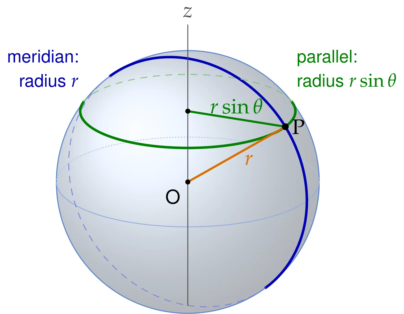
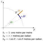
A scale factor converts "how much did the coordinate change" into "how many metres did the point move". The radial distance is already a length (). An angle is not: one radian of is an arc of the meridian, which has radius , but one radian of is an arc of the parallel, which has the smaller radius (Figure 2.3.20). Near the poles the parallels shrink to points, so changing there hardly moves P at all.
It is worth checking that these vectors really form an orthonormal, right-handed triple. Each has unit length by construction. Their mutual dot products vanish, e.g.
and similarly . A short computation of the cross product gives
so the order is right-handed, just like and . The order matters: in formulas such as the curl determinant of Section 2.3.10, the coordinates must always be listed as .
Comparing Eq. (2.3.34) with Eq. (2.3.31) we notice that : in spherical coordinates the position vector has a single component. The information about the direction of P, i.e. about and , is hidden inside the unit vector itself. This brings us to the most important practical difference between Cartesian and curvilinear coordinates.
A point P has and . How far does P move if (i) increases by , (ii) increases by ? What happens to (ii) at the north pole?
(i) . (ii) . At the north pole : changing does not move the point at all, which is why is undefined there.
The unit vectors depend on position
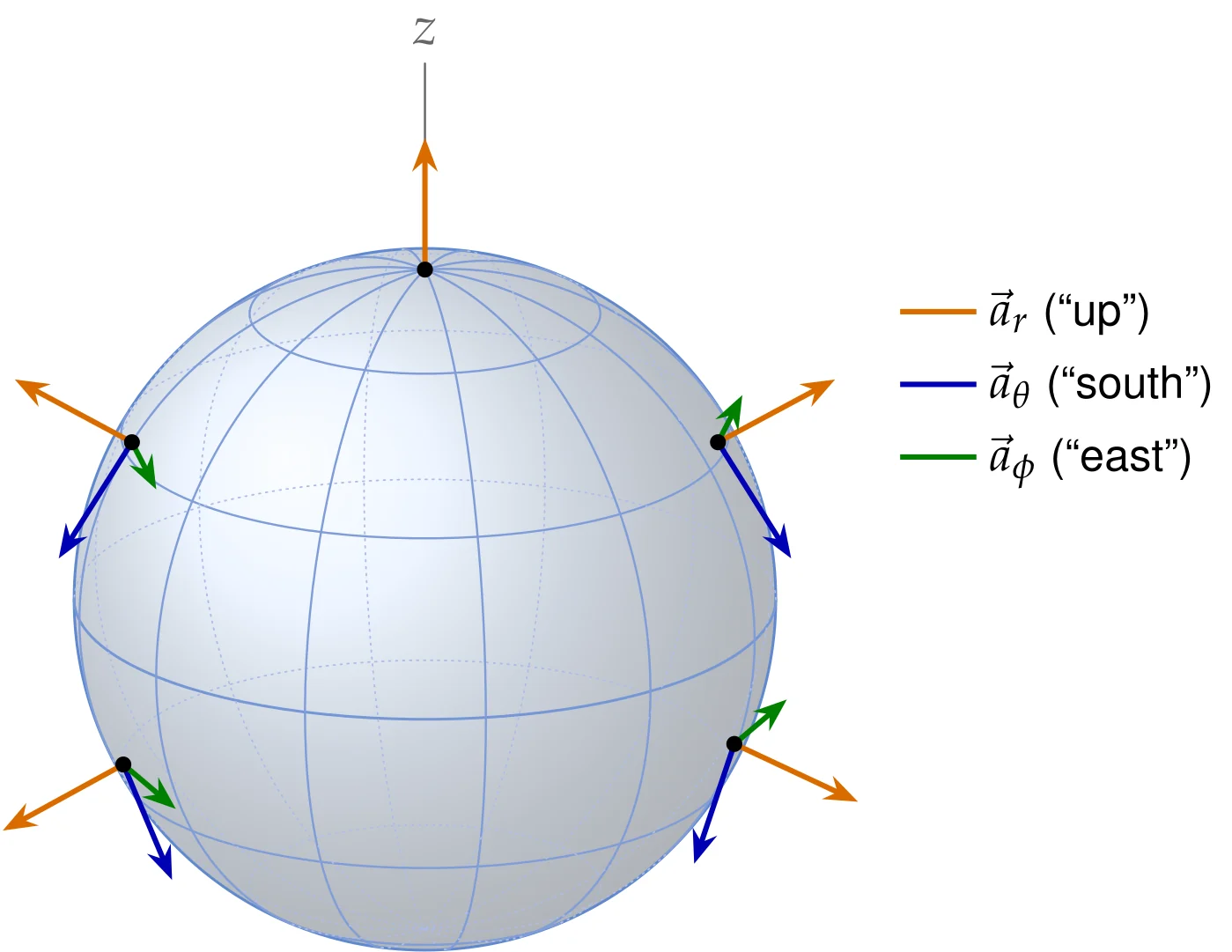
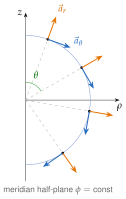
The Cartesian unit vectors point the same way everywhere. The spherical unit vectors do not: at the north pole is , while on the positive axis is . On the globe, is "up" (towards the sky), is "south" and is "east". But "up", "south" and "east" in Ankara are different directions in space from "up", "south" and "east" in Tokyo. Figure 2.3.21 shows the triad at several points of a sphere, and Figure 2.3.22(a) shows and along one meridian. They turn as the point moves.
Differentiating Eqs. (2.3.34) to (2.3.36) and re-expressing the results in the spherical unit vectors gives
For instance, : tilting the direction southwards turns "up" towards "south". None of the unit vectors changes along the radial direction (moving outwards along a ray does not turn anything), but all of them change with the angles.
Two consequences will accompany us through the whole course.
-
Differentiation. When we differentiate a vector field written in spherical (or cylindrical) components, the unit vectors must be differentiated too. This is why the operator formulas of Section 2.3.10 contain extra factors such as and : they are the fingerprints of Eq. (2.3.38).
-
Integration. A unit vector such as may not be taken outside an integral over a region in which it changes direction. For example, integrating over a sphere of radius centred at the origin does not give (which would not even be well defined: at which point is that evaluated?). Writing in Cartesian form, Eq. (2.3.34), whose unit vectors are constant, and using (see Eq. (2.3.40) below),
because and . Physically: the outward directions on opposite sides of the sphere cancel. The rule is simple. Before integrating a vector, convert its unit vectors to Cartesian ones. (Scalar integrands, such as a flux , have no such problem.)
Adding or integrating unit vectors that belong to different points as if they were the same vector, e.g. writing , or pulling , , (or , ) out of an integral. Only , , are the same everywhere.
Write , and in Cartesian unit vectors at the point where the positive axis pierces a sphere (, ).
From Eqs. (2.3.34) to (2.3.36): , , . (Check: .)
Differential elements of length, surface and volume
With the scale factors at hand, the general formula of Section 2.3.2, , gives the differential length
Each term has the dimension of length: is a radial step, an arc along a meridian of radius , and an arc along a parallel of radius . The angles themselves are dimensionless, so it is the scale factors that carry the metres.
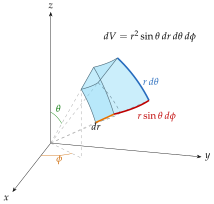
Let the three coordinates increase by , , . The point P then sweeps out the small "curved brick" of Figure 2.3.23, bounded by two spheres, two cones and two half-planes. Since the surfaces are mutually orthogonal, its edges , and are mutually perpendicular, and to first order the brick is a rectangular box. Its faces give the differential surface elements (the vector is normal to the face, with magnitude equal to its area):
where the sign is chosen according to the required orientation (for a closed surface: outwards). Each area is simply the product of the two edges that lie in that face: on the sphere the edges are and , and so on. The volume is the product of all three edges,
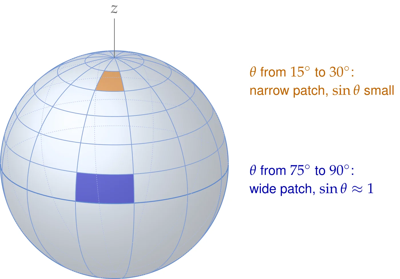
The factor is the Jacobian of the transformation, Eq. (2.3.30). It expresses two simple geometric facts: bricks of the same are larger far from the origin (factor ), and they are thinner near the poles, where the parallels shrink to a point (factor ). Figure 2.3.24 shows the second fact on a globe.
Forgetting the factor and writing "" (or "" on a sphere). Besides giving wrong numbers, such an element does not even have the units of a volume (or an area): and are dimensionless. A quick unit check catches this error every time.
Which surface element do you need to find the area of the curved surface of a cone between its apex and the slant distance ? What is the area?
On the cone , so . This is the familiar .