Electromagnetic Fields and Waves: Notes, Solved Problems and Interactive Lab

A vector at a point can be expressed in either system:

A = A_{x} a_{x} + A_{y} a_{y} + A_{z} a_{z} = A_{ρ} a_{ρ} + A_{ϕ} a_{ϕ} + A_{z} a_{z} . (2.3.27)

The vector itself is the same arrow. Only the set of unit vectors used to describe it differs (Figure 2.3.13). Since the unit vectors of each system are orthonormal, each component is a projection (Section 2.1): $A_{ρ} = A \cdot a_{ρ}$ , $A_{ϕ} = A \cdot a_{ϕ}$ , $A_{x} = A \cdot a_{x}$ , $A_{y} = A \cdot a_{y}$ . The dot products between the unit vectors of the two systems follow from Eqs. (2.3.19) and (2.3.20) and are collected in Table 2.3.2.

$One vector, two sets of components (top view). At the point \mathrm P, whose angle is \phi, the cylindrical unit vectors \vec a_\rho,\vec a_\phi are the Cartesian ones \vec a_x,\vec a_y rotated by \phi (only \vec a_x is drawn, in grey). The same arrow \vec A projects onto \vec a_\rho and \vec a_\phi (coloured bars) to give A_\rho and A_\phi, and onto \vec a_x and \vec a_y to give A_x and A_y.$

Figure 2.3.13. One vector, two sets of components (top view). At the point

P

, whose angle is

ϕ

, the cylindrical unit vectors

a_{ρ}, a_{ϕ}

are the Cartesian ones

a_{x}, a_{y}

rotated by

ϕ

(only

a_{x}

is drawn, in grey). The same arrow

A

projects onto

a_{ρ}

and

a_{ϕ}

(coloured bars) to give

A_{ρ}

and

A_{ϕ}

, and onto

a_{x}

and

a_{y}

to give

A_{x}

and

A_{y}

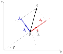
Table 2.3.2. Dot products of Cartesian and cylindrical unit vectors.

$\cdot$	$a_{ρ}$	$a_{ϕ}$	$a_{z}$
$a_{x}$	$cos ϕ$	$- sin ϕ$	$0$
$a_{y}$	$sin ϕ$	$cos ϕ$	$0$
$a_{z}$	$0$	$0$	$1$

Taking the dot product of Eq. (2.3.27) with $a_{ρ}$ and with $a_{ϕ}$ ,

A_{ρ} A_{ϕ} = A_{x} a_{x} \cdot a_{ρ} + A_{y} a_{y} \cdot a_{ρ} = A_{x} cos ϕ + A_{y} sin ϕ, = - A_{x} sin ϕ + A_{y} cos ϕ,

while $A_{z}$ is common to both systems. In matrix form, the conversion between Cartesian and cylindrical components of a vector $A$ is

Conversion of vector components

A_{ρ} A_{ϕ} A_{z} = cos ϕ - sin ϕ 0 sin ϕ cos ϕ 0 001 A_{x} A_{y} A_{z}, (2.3.28)

A_{x} A_{y} A_{z} = cos ϕ sin ϕ 0 - sin ϕ cos ϕ 0 001 A_{ρ} A_{ϕ} A_{z} . (2.3.29)

The two matrices are transposes of each other and their product is the identity matrix: the transformation is a rotation by the angle $ϕ$ about the $z$ -axis, which preserves lengths, so $A_{ρ}^{2} + A_{ϕ}^{2} + A_{z}^{2} = A_{x}^{2} + A_{y}^{2} + A_{z}^{2}$ .

Recipe · Converting a vector field from Cartesian to cylindrical coordinates

Transform the components with Eq. (2.3.28): $A_{ρ} = A_{x} cos ϕ + A_{y} sin ϕ$ , $A_{ϕ} = - A_{x} sin ϕ + A_{y} cos ϕ$ , $A_{z}$ unchanged.
Replace the coordinates in the expressions: $x = ρ cos ϕ$ , $y = ρ sin ϕ$ (Eq. (2.3.15)).
Simplify (often with $sin^{2} ϕ + cos^{2} ϕ = 1$ ), and check that the magnitude is unchanged.

For a single vector located at a given point, use the angle $ϕ$ of that point. The reverse conversion uses Eqs. (2.3.29) and (2.3.16).

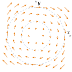
For example, for $A = y a_{x} - x a_{y}$ ,

A_{ρ} A_{ϕ} = y cos ϕ - x sin ϕ = ρ sin ϕ cos ϕ - ρ cos ϕ sin ϕ = 0, = - y sin ϕ - x cos ϕ = - ρ (sin^{2} ϕ + cos^{2} ϕ) = - ρ,

so $A = - ρ a_{ϕ}$ : a field circulating clockwise around the $z$ -axis with a strength proportional to the distance from it (Figure 2.3.14), which is far from obvious in the Cartesian form. Note that $ϕ$ in the conversion matrix is the angle of the point at which the vector is located, and for a vector field it varies from point to point.

The field \vec A=y\,\vec a_x-x\,\vec a_y (computed on a grid). In cylindrical coordinates it is simply \vec A=-\rho\,\vec a_\phi: on every circle around the z-axis (dashed) the arrows are tangent, point clockwise (against increasing \phi), and have the same length \rho, twice as long on the outer circle as on the inner one. — **Figure 2.3.14.** The field $A = y a_{x} - x a_{y}$ (computed on a grid). In cylindrical coordinates it is simply $A = - ρ a_{ϕ}$ : on every circle around the $z$ -axis (dashed) the arrows are tangent, point clockwise (against increasing $ϕ$ ), and have the same length $ρ$ , twice as long on the outer circle as on the inner one.

Common mistake

Converting only the components and forgetting the coordinates (or the other way round). After step 1 of the recipe the expressions still contain $x$ and $y$ , but a vector field in cylindrical coordinates must be written with $ρ$ , $ϕ$ , $z$ only. Conversely, a cylindrical expression like $- ρ a_{ϕ}$ is not converted to Cartesian form by replacing $ρ$ with $x^{2} + y^{2}$ alone: $a_{ϕ}$ must be replaced as well.

Table 2.3.3 summarises the two systems side by side.

Table 2.3.3. The two coordinate systems of this section at a glance.

	Cartesian $(x, y, z)$	Cylindrical $(ρ, ϕ, z)$
ranges	$- \infty < x, y, z < \infty$	$ρ \geq 0$ , $0 \leq ϕ < 2 π$ , $- \infty < z < \infty$
position vector	$x a_{x} + y a_{y} + z a_{z}$	$ρ a_{ρ} + z a_{z}$
scale factors	$1, 1, 1$	$1, ρ, 1$
$d ℓ$	$d x a_{x} + d y a_{y} + d z a_{z}$	$d ρ a_{ρ} + ρ d ϕ a_{ϕ} + d z a_{z}$
$d S$	$d y d z a_{x}$ , $d z d x a_{y}$ , $d x d y a_{z}$	$ρ d ϕ d z a_{ρ}$ , $d ρ d z a_{ϕ}$ , $ρ d ρ d ϕ a_{z}$
$d V$	$d x d y d z$	$ρ d ρ d ϕ d z$
unit vectors	constant	$a_{ρ}, a_{ϕ}$ depend on $ϕ$

Integration in cylindrical coordinates

The following examples use the cylindrical elements (2.3.24) to (2.3.26). In each one the surface or volume is bounded by coordinate surfaces of the cylindrical system, so the limits are constants, whereas in Cartesian coordinates they would be functions such as $y = \pm b^{2} - x^{2}$ .

Example 2.3.11Circumference of a circle Example 2.3.12Area of a circle Example 2.3.13Lateral area of a cylinder Example 2.3.14Volume of a cylinder Example 2.3.15A closed line integral in cylindrical coordinates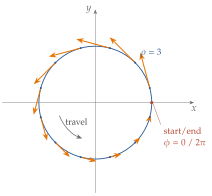

The path and the field of Example 2.3.15. The circle \rho=3 is traversed counter-clockwise (direction of \vec a_\phi). The arrows show \vec A=4\rho\cos(\phi/4)\,\vec a_\phi at \phi=15^\circ,45^\circ,\dots,345^\circ, drawn to scale: tangent to the path, shrinking from almost 4\rho=12 just after \phi=0 to nearly zero just before \phi=2\pi. Every contribution \vec A\cdot d\vec\ell is positive, so the circulation is positive. The field jumps across the half-plane \phi=0 (red dot). — **Figure 2.3.15.** The path and the field of Example 2.3.15. The circle $ρ = 3$ is traversed counter-clockwise (direction of $a_{ϕ}$ ). The arrows show $A = 4 ρ cos (ϕ /4) a_{ϕ}$ at $ϕ = 1 5^{\circ}, 4 5^{\circ}, \dots, 34 5^{\circ}$ , drawn to scale: tangent to the path, shrinking from almost $4 ρ = 12$ just after $ϕ = 0$ to nearly zero just before $ϕ = 2 π$ . Every contribution $A \cdot d ℓ$ is positive, so the circulation is positive. The field jumps across the half-plane $ϕ = 0$ (red dot).

Looking ahead

Three ideas of the first part of this section carry the rest of the course: the position and displacement vectors $r$ , $r^{'}$ and $R = r - r^{'}$ , the scale factors $h_{i}$ , and the habit of reducing every line, surface and volume integral to ordinary integrals with constant limits by choosing coordinates that fit the geometry. With nothing more than these, Section 2.3.6 develops spherical coordinates, Section 2.3.10 writes the gradient, divergence, curl and Laplacian in curvilinear coordinates, and Section 2.4 turns the definitions of divergence and curl into the integral theorems of Gauss and Stokes.

2.3.5 Cartesian vs. cylindrical coordinates

Integration in cylindrical coordinates

In this part

Examples · 5