Electromagnetic Fields and Waves: Notes, Solved Problems and Interactive Lab

A vector field is a physical object, while the coordinate system is only our choice of description. The same vector $A$ at a point P can therefore be written in any of the three systems, and we must be able to translate between them. Two different things have to be converted:

the coordinates of the point at which the vector is evaluated, e.g. $(x, y, z) \to (r, θ, ϕ)$ by Eqs. (2.3.30) to (2.3.32), and
the components of the vector, e.g. $(A_{x}, A_{y}, A_{z}) \to (A_{r}, A_{θ}, A_{ϕ})$ , which is the subject of this subsection.

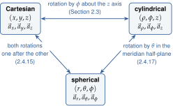
Figure 2.3.26 is a map of all the conversions we need. The Cartesian to cylindrical one was derived in Section 2.3.4.

The conversions between the three coordinate systems. Each conversion of vector components is a rotation of the unit-vector triad, described by an orthogonal 3\times3 matrix whose entries depend on the point (on \phi, on \theta, or on both). Going from Cartesian to spherical directly or via cylindrical gives the same result. — **Figure 2.3.26.** The conversions between the three coordinate systems. Each conversion of vector components is a rotation of the unit-vector triad, described by an orthogonal $3 \times 3$ matrix whose entries depend on the point (on $ϕ$ , on $θ$ , or on both). Going from Cartesian to spherical directly or via cylindrical gives the same result.

Cartesian and spherical components

Write the same vector in both bases:

A = A_{x} a_{x} + A_{y} a_{y} + A_{z} a_{z} = A_{r} a_{r} + A_{θ} a_{θ} + A_{ϕ} a_{ϕ} . (2.3.43)

Because the spherical unit vectors are orthonormal, each spherical component is obtained by projection. Dotting Eq. (2.3.43) with $a_{r}$ kills the $a_{θ}$ and $a_{ϕ}$ terms on the right and leaves $A_{r} = A \cdot a_{r} = A_{x} (a_{x} \cdot a_{r}) + A_{y} (a_{y} \cdot a_{r}) + A_{z} (a_{z} \cdot a_{r})$ , and similarly for $A_{θ}$ and $A_{ϕ}$ . The dot products $a_{x} \cdot a_{r} = sin θ cos ϕ$ , etc., are just the Cartesian components of the spherical unit vectors listed in Eqs. (2.3.34) to (2.3.36). In matrix form:

Cartesian ↔ spherical

A_{r} A_{θ} A_{ϕ} = sin θ cos ϕ cos θ cos ϕ - sin ϕ sin θ sin ϕ cos θ sin ϕ cos ϕ cos θ - sin θ 0 A_{x} A_{y} A_{z}, A_{x} A_{y} A_{z} = sin θ cos ϕ sin θ sin ϕ cos θ cos θ cos ϕ cos θ sin ϕ - sin θ - sin ϕ cos ϕ 0 A_{r} A_{θ} A_{ϕ} . (2.3.44)

The rows of the first matrix are the Cartesian components of $a_{r}$ , $a_{θ}$ and $a_{ϕ}$ , so you do not need to memorise it: it is Eqs. (2.3.34) to (2.3.36) written as a table. Because these three rows are orthonormal vectors, the matrix is orthogonal: its inverse is simply its transpose, which is the second matrix of Eq. (2.3.44). (Its columns, read downwards, are the spherical components of $a_{x}$ , $a_{y}$ , $a_{z}$ . For instance, $a_{z} = cos θ a_{r} - sin θ a_{θ}$ .) An orthogonal transformation preserves lengths and angles, so $A_{x}^{2} + A_{y}^{2} + A_{z}^{2} = A_{r}^{2} + A_{θ}^{2} + A_{ϕ}^{2}$ , as it must: the magnitude of a vector cannot depend on the basis used to describe it.

The matrix entries depend on $θ$ and $ϕ$ , i.e. on where the vector is attached. To convert a vector field, we therefore apply Eq. (2.3.44) at every point and also express the coordinates themselves in the new system. As an illustration, take the position vector $r = x a_{x} + y a_{y} + z a_{z}$ , i.e. $A_{x} = x$ , $A_{y} = y$ , $A_{z} = z$ , and use Eq. (2.3.30):

A_{r} = sin θ cos ϕ (r sin θ cos ϕ) + sin θ sin ϕ (r sin θ sin ϕ) + cos θ (r cos θ) = r,

A_{θ} A_{ϕ} = r (cos θ sin θ cos^{2} ϕ + cos θ sin θ sin^{2} ϕ - sin θ cos θ) = 0, = r sin θ (- sin ϕ cos ϕ + cos ϕ sin ϕ) = 0,

so $r = r a_{r}$ , in agreement with the subsection on unit vectors and scale factors above.

Recipe · Converting a vector field between coordinate systems

Read off the old components (e.g. $A_{x}, A_{y}, A_{z}$ ) as functions of the old coordinates.
Multiply by the conversion matrix, whose entries are evaluated at the point where the vector sits. This is Eq. (2.3.44), Eq. (2.3.46) or the Cartesian to cylindrical matrix of Section 2.3.
Replace the old coordinates by the new ones, e.g. $x = r sin θ cos ϕ$ , … from Eq. (2.3.30).
Simplify, and check that the magnitude has not changed: $A_{x}^{2} + A_{y}^{2} + A_{z}^{2} = A_{r}^{2} + A_{θ}^{2} + A_{ϕ}^{2}$ .

Common mistake

Converting the components but forgetting step 3, which leaves a "mixed" answer such as $A_{r} = x sin θ cos ϕ + \dots$ with Cartesian coordinates inside spherical components. Both the components and the coordinates must be converted.

Quick check

Express the Cartesian unit vector $a_{x}$ in spherical components at a point on the positive $y$ axis ( $θ = π /2$ , $ϕ = π /2$ ). Then do the same at a point on the positive $x$ axis.

With $(A_{x}, A_{y}, A_{z}) = (1, 0, 0)$ , the first column of the first matrix gives $(A_{r}, A_{θ}, A_{ϕ}) = (sin θ cos ϕ, cos θ cos ϕ, - sin ϕ)$ . On the $+ y$ axis this is $(0, 0, - 1)$ , so $a_{x} = - a_{ϕ}$ there. On the $+ x$ axis ( $θ = π /2$ , $ϕ = 0$ ) it is $(1, 0, 0)$ , so $a_{x} = a_{r}$ . Same vector, different components at different points.

Cylindrical and spherical components

Cylindrical and spherical coordinates share the azimuth $ϕ$ and the unit vector $a_{ϕ}$ . In a meridian half-plane $ϕ = const$ (Figure 2.3.22(b)) the remaining coordinates are related by elementary trigonometry,

ρ = r sin θ, z = r cos θ, r = ρ^{2} + z^{2}, θ = arccos \frac{z}{ρ ^{2} + z ^{2}}, (2.3.45)

and the unit-vector pair $(a_{θ}, a_{r})$ is the pair $(a_{ρ}, a_{z})$ rotated by $θ$ ( $a_{r}$ makes the angle $θ$ with $a_{z}$ , and $a_{θ}$ with $a_{ρ}$ ):

a_{r} a_{θ} a_{ϕ} = sin θ a_{ρ} + cos θ a_{z}, = cos θ a_{ρ} - sin θ a_{z}, = a_{ϕ} .

(One can confirm this by substituting $a_{ρ} = cos ϕ a_{x} + sin ϕ a_{y}$ from Section 2.3.4 into the right-hand sides and comparing with Eqs. (2.3.34) and (2.3.35).) Writing the same vector in both bases, $A = A_{ρ} a_{ρ} + A_{ϕ} a_{ϕ} + A_{z} a_{z} = A_{r} a_{r} + A_{θ} a_{θ} + A_{ϕ} a_{ϕ}$ , and projecting onto the unit vectors as before, we obtain:

Cylindrical ↔ spherical

A_{r} A_{θ} A_{ϕ} = sin θ cos θ 0 001 cos θ - sin θ 0 A_{ρ} A_{ϕ} A_{z}, A_{ρ} A_{ϕ} A_{z} = sin θ 0 cos θ cos θ 0 - sin θ 010 A_{r} A_{θ} A_{ϕ} . (2.3.46)

Again the second matrix is the transpose of the first. Note that these matrices depend only on $θ$ . The three transformations fit together consistently: multiplying the cylindrical to spherical matrix of Eq. (2.3.46) by the Cartesian to cylindrical matrix of Section 2.3,

sin θ cos θ 0 001 cos θ - sin θ 0 cos ϕ - sin ϕ 0 sin ϕ cos ϕ 0 001

= sin θ cos ϕ cos θ cos ϕ - sin ϕ sin θ sin ϕ cos θ sin ϕ cos ϕ cos θ - sin θ 0,

reproduces the Cartesian to spherical matrix of Eq. (2.3.44): going from Cartesian to spherical components directly or via cylindrical components gives the same answer (Figure 2.3.26).

Quick check

Write the cylindrical unit vector $a_{z}$ in spherical components. At which points is it equal to $a_{r}$ , and where is it equal to $- a_{θ}$ ?

Put $(A_{ρ}, A_{ϕ}, A_{z}) = (0, 0, 1)$ into Eq. (2.3.46): $a_{z} = cos θ a_{r} - sin θ a_{θ}$ . It equals $a_{r}$ on the positive $z$ axis ( $θ = 0$ ) and $- a_{θ}$ in the $x y$ -plane ( $θ = π /2$ ).

2.3.8 Transformations between coordinate systems

Cartesian and spherical components

Cylindrical and spherical components