Electromagnetic Fields and Waves: Notes, Solved Problems and Interactive Lab

Inner currents and the magnetic polarisation M

Just as in electrostatics, magnetostatic phenomena may differ in media other than free space. If the medium is magnetic, its inner charges, the electrons bound to the atoms, may gain a velocity due to the external sources, and moving charges are currents. For free space the first fundamental equation of magnetostatics (Section 4.1) reads

\nabla \times \frac{B}{μ _{0}} = J, (4.2.1)

where $J$ is the current density of the sources we control, the free current in the wires. Now suppose the medium contains inner charges that have been set in motion as described above. If we express the additional current density due to these charges as $J_{m}$ , the field they produce obeys the same law as the field of any other current, and so

\nabla \times \frac{B}{μ _{0}} = J + J_{m} . (4.2.2)

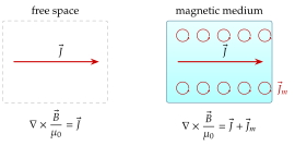
Figure 4.2.1 shows the two situations side by side. The trouble with Eq. (4.2.2) is that $J_{m}$ is not something we know in advance: it is the material's answer to the field, exactly as the bound charge $ρ_{b}$ of Section 3.4 was.

The same free current \vec J in free space (left) and in a magnetic medium (right). In the medium the atomic current loops (small red circles) are set in order by the field and add their own current density \vec J_m to the source of \vec B. — **Figure 4.2.1.** The same free current $J$ in free space (left) and in a magnetic medium (right). In the medium the atomic current loops (small red circles) are set in order by the field and add their own current density $J_{m}$ to the source of $B$ .

The way out is the same as in electrostatics: describe the material's answer by a vector field of its own and move it to the left-hand side. We define the magnetic polarisation vector $M$ such that

J_{m} = \nabla \times (\frac{M}{μ _{0}}) . (4.2.3)

Substituting into Eq. (4.2.2),

⟹ \nabla \times (\frac{B}{μ _{0}}) = J + \nabla \times (\frac{M}{μ _{0}}) \nabla \times (\frac{B - M}{μ _{0}}) = J .

The vector in the brackets has the free current, and only the free current, as its curl. Since $\nabla \times H = J$ is satisfied universally, in every medium, this vector must be the magnetic field intensity $H$ , and we determine

The constitutive relation of a magnetic medium

B = μ_{0} H + M [T] . (4.2.4)

In plain words

$H$ is made by the currents in the wires, $M$ is what the material adds, and $B$ , the field that pushes on charges, is the sum of the two. Compare $D = ε_{0} E + P$ of Section 3.4: there the material added to the flux density, here it adds to the magnetic flux density $B$ .

Units of M

In this book, following the lectures, $M$ is defined so that it carries the units of $B$ , tesla, and Eq. (4.2.4) has no factor in front of $M$ . Many texts define a magnetisation $M^{'} = M / μ_{0}$ in A/m, the dipole moment per unit volume, and write $B = μ_{0} (H + M^{'})$ . The physics is the same. Whenever a magnetisation in A/m is wanted, it is $M / μ_{0}$ .

What M describes: aligned atomic loops and the bound currents

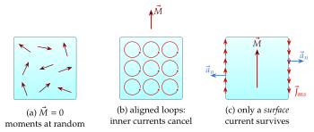
Each atom carries a tiny circulating current, a magnetic dipole (Section 4.2.8 shows that a small current loop is a dipole). Without a field the moments point at random and cancel (Figure 4.2.2a). An applied $H$ lines them up (Figure 4.2.2b). $M$ is the dipole moment per unit volume, times $μ_{0}$ so that it has the units of $B$ . Inside the body, neighbouring loops carry their currents in opposite directions along their common edge, so the inner currents cancel, and what is left of all the aligned loops is a current flowing round the surface of the body (Figure 4.2.2c). Where $M$ is not uniform the cancellation inside is incomplete and a volume current remains. In formulae,

J_{m} J_{m s} = \nabla \times \frac{M}{μ _{0}} in V [A/ m^{2}], = \frac{1}{μ _{0}} M \times a_{n} on S [A/m], (4.2.5)

where $a_{n}$ is the outward normal of the surface S of the body. These are the bound (or magnetisation) currents, the magnetic counterparts of the bound charges $ρ_{b} = - \nabla \cdot P$ and $ρ_{S b} = P \cdot a_{n}$ of Section 3.4.

What \vec M describes. (a) Without a field the atomic moments point at random and \vec M=0. (b) An applied field aligns the atomic current loops. Along every edge shared by two neighbouring loops the currents run in opposite directions and cancel. (c) What survives is a current sheet \vec J_{ms}=\vec M\times\vec a_n/\mu_0 on the surface of the body, running round it like the winding of a solenoid. — **Figure 4.2.2.** What $M$ describes. (a) Without a field the atomic moments point at random and $M = 0$ . (b) An applied field aligns the atomic current loops. Along every edge shared by two neighbouring loops the currents run in opposite directions and cancel. (c) What survives is a current sheet $J_{m s} = M \times a_{n} / μ_{0}$ on the surface of the body, running round it like the winding of a solenoid.

Why it matters

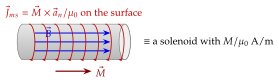
$J_{m}$ is not a current you can put an ammeter in: no charge is carried from one place to another, each electron stays with its atom. Yet it makes a field exactly like a real current. A uniformly magnetised cylinder (a bar magnet) is, seen from outside, indistinguishable from a solenoid of the same size carrying $M / μ_{0}$ ampere-turns per metre (Figure 4.2.3): by Eq. (4.2.5), with $M = M a_{z}$ and $a_{n} = a_{ρ}$ on the curved surface, $J_{m s} = (M / μ_{0}) a_{z} \times a_{ρ} = (M / μ_{0}) a_{ϕ}$ , a sheet current circulating round the cylinder, while on the flat end faces $a_{n} = \pm a_{z}$ is parallel to $M$ and $J_{m s} = 0$ . For $M = 1.2 T$ the sheet carries $M / μ_{0} = 1.2/ (4 π \times 1 0^{- 7}) = 9.55 \times 1 0^{5} A/m$ (Exercise 4.2.1): a bar magnet is a solenoid with nearly a million ampere-turns per metre, and no battery.

A uniformly magnetised cylinder. Inside, the aligned atomic loops cancel and \vec J_m=0. On the curved surface the bound sheet current \vec J_{ms}=(M/\mu_0)\vec a_\phi survives, so the cylinder produces the field of a solenoid carrying M/\mu_0 ampere-turns per metre. — **Figure 4.2.3.** A uniformly magnetised cylinder. Inside, the aligned atomic loops cancel and $J_{m} = 0$ . On the curved surface the bound sheet current $J_{m s} = (M / μ_{0}) a_{ϕ}$ survives, so the cylinder produces the field of a solenoid carrying $M / μ_{0}$ ampere-turns per metre.

Bound currents and H: the bookkeeping

The two fields now have distinct jobs. $B$ comes from all currents, free and bound, and it is $B$ that enters the Lorentz force. $H$ comes from the free current only, so $\nabla \times H = J$ holds in every medium, which is why $H$ , not $B$ , appears in Ampère's law. This is the engineering point of view adopted throughout this book: we work with the field intensity $H$ , which the currents in our wires fix directly, and derive $B$ from it through the material.

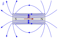
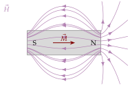
Figure 4.2.4 makes the distinction visible for a bar magnet, computed from Eq. (4.2.4). Outside the magnet there is no $M$ and the two fields are proportional, $B = μ_{0} H$ : the lines are the same. Inside, $B$ runs from the S end to the N end and its lines close on themselves, as $\nabla \cdot B = 0$ demands. $H$ , on the other hand, has no free current to circulate around: its lines begin on the N face and end on the S face, outside and inside, so that inside the magnet $H$ points against $M$ . This inner field is called the demagnetising field. In a long thin magnet it is small (about $- 0.05 M / μ_{0}$ at the centre of the rod of the figure, whose length is three times its diameter), in a short fat one it is large, which is why a short magnet needs a material that resists demagnetisation, a permanent-magnet material (Exercise 4.2.1).

Left: the lines of \vec B. — Left: the lines of $B$ .

Right: the lines of \vec H. Computed field lines of a uniformly magnetised rod (length three times the diameter, section through the axis, \vec M to the right). Left: the lines of \vec B are closed and run through the magnet from S to N. Most of them leave and enter through the end faces, a few through the sides near the ends. Right: the lines of \vec H start on the N face and end on the S face, outside the magnet exactly like those of \vec B (there \vec B=\mu_0\vec H), but inside they run *against* \vec M: the demagnetising field. — **Figure 4.2.4.** Right: the lines of $H$ . Computed field lines of a uniformly magnetised rod (length three times the diameter, section through the axis, $M$ to the right). Left: the lines of $B$ are closed and run through the magnet from S to N. Most of them leave and enter through the end faces, a few through the sides near the ends. Right: the lines of $H$ start on the N face and end on the S face, outside the magnet exactly like those of $B$ (there $B = μ_{0} H$ ), but inside they run *against* $M$ : the demagnetising field.

Quick check

A long rod is uniformly magnetised with $M = 0.8 a_{z} T$ . What is the bound surface current density on its curved surface, and what is the bound volume current density inside?

$J_{m s} = M \times a_{ρ} / μ_{0} = (0.8/4 π \times 1 0^{- 7}) a_{ϕ} = 6.37 \times 1 0^{5} a_{ϕ} A/m$ , and $J_{m} = \nabla \times M / μ_{0} = 0$ because $M$ is uniform.

Susceptibility and relative permeability

For most materials the magnetisation is proportional to the field intensity that produces it. The magnetic polarisation vector $M$ is considered to be related to the magnetic field by

M = μ_{0} χ_{m} H, (4.2.6)

where the dimensionless number $χ_{m}$ is the magnetic susceptibility of the medium. This yields, with Eq. (4.2.4),

B = μ_{0} H + μ_{0} χ_{m} H = μ_{0} (1 + χ_{m}) H .

Defining the relative permeability as

μ_{r} = 1 + χ_{m}, (4.2.7)

we find

Permeability of a medium

B = μ H, μ = μ_{0} μ_{r} [H/m] (4.2.8)

as the permeability of the medium. In free space $μ_{r} = 1$ and $μ = μ_{0} = 4 π \times 1 0^{- 7} H/m$ .

In plain words

$μ_{r}$ says by how much the material multiplies the flux density that a given winding current produces: the winding fixes $H$ , and the material supplies $μ_{r}$ times the $B$ of free space. In air $μ_{r}$ is $1$ to five decimal places, in iron it can be thousands.

A material with $M = μ_{0} χ_{m} H$ is called linear, and if $χ_{m}$ is the same at every point and in every direction, homogeneous and isotropic. For such a simple medium the whole effect of the material is the single number $μ_{r}$ , exactly as $ε_{r}$ summarised a simple dielectric. Exercise 4.2.2 works the three quantities $H$ , $B$ and $M$ out for a solenoid filled with air, with a paramagnetic salt and with soft iron.

Common mistake · Mixing up what the winding fixes

It is $H$ that Ampère's law ties to the winding current, not $B$ . Filling a solenoid with iron does not change $H = n I$ at all. It changes $B$ , by the factor $μ_{r}$ , and the extra flux is supplied by the bound surface current of the iron, not by the winding.

Classification of magnetic materials

Although $ε_{r}$ in electrostatics was found to be always greater than $1$ , $μ_{r}$ in magnetostatics can have values lower than $1$ as well. Magnetic materials are roughly classified into three groups (Figure 4.2.5):

Diamagnetic materials ( $μ_{r} ≲ 1$ , $χ_{m} < 0$ ): the induced atomic currents oppose the applied field, which is slightly weakened. Copper, bismuth, water.
Paramagnetic materials ( $μ_{r} ≳ 1$ , $χ_{m} > 0$ and small): the atoms carry permanent moments that align weakly with the field. Aluminium, platinum, air.
Ferromagnetic materials ( $μ_{r} ≫ 1$ ): iron, nickel, cobalt and their alloys, and the ferrites (ferrimagnetic ceramics).

In fact, most materials have $μ_{r}$ values very close to $1$ . For aluminium it is $μ_{r} = 1.000022$ , while for copper it is $μ_{r} = 0.999994$ . For almost every engineering purpose such materials behave like free space. Ferromagnetic materials, however, have very large relative permeabilities and their magnetic properties are quite interesting, which is the subject of Application 4.2.1.

The three classes of magnetic materials on a logarithmic \mu_r axis. Diamagnetic and paramagnetic materials sit within a few parts in 10^{5} of \mu_r=1 on either side. The ferromagnetic materials are two to five orders of magnitude away. — **Figure 4.2.5.** The three classes of magnetic materials on a logarithmic $μ_{r}$ axis. Diamagnetic and paramagnetic materials sit within a few parts in $1 0^{5}$ of $μ_{r} = 1$ on either side. The ferromagnetic materials are two to five orders of magnitude away.

Quick check

A solenoid produces $H = 4000 A/m$ . What is $B$ with an air core, and with a copper core ( $μ_{r} = 0.999994$ )?

$B = μ_{0} H = 4 π \times 1 0^{- 7} \times 4000 = 5.027 mT$ in air. Copper lowers it by $6$ parts in a million, to $5.02652 mT$ instead of $5.02655 mT$ : for any practical purpose copper is magnetically the same as air.

Application 4.2.1 · Ferromagnetic materials and the relative permeability

In a ferromagnet the atomic moments align spontaneously, in regions called domains, even without an applied field. In an unmagnetised piece of iron the domains point in all directions and cancel. An applied $H$ grows the favourably oriented domains at the expense of the others, so a tiny $H$ produces a huge $M$ , and the relation between $B$ and $H$ is not linear (Figure 4.2.6): $μ_{r} = 1 + χ_{m}$ is a local slope of the $B (H)$ curve, not a constant. Three features of the curve matter in practice.

$B$ saturates. Once all domains are aligned, $M$ can grow no further and $B$ rises only as $μ_{0} H$ , as in air. The saturation flux density is $B_{s} \approx 2.1 T$ for iron and about $0.35$ – $0.5 T$ for manganese-zinc ferrite. Past $B_{s}$ the core behaves like air.
The curve shows hysteresis: on reducing $H$ to zero a remanent flux density $B_{r}$ stays (this is what a permanent magnet is), and a reverse coercive field $H_{c}$ is needed to bring $B$ back to zero. The area of the loop is the hysteresis loss per cycle per unit volume, paid $f$ times a second in a core driven at the frequency $f$ .
Above the Curie temperature the thermal agitation destroys the domains and $μ_{r} \to 1$ : $770^{\circ} C$ for iron, $358^{\circ} C$ for nickel, $1115^{\circ} C$ for cobalt.

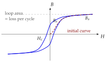
The B(H) curve of a ferromagnet. The dashed initial curve starts from the unmagnetised state and bends over at the saturation flux density B_s. Cycling H traces the hysteresis loop, which crosses the B axis at the remanence B_r and the H axis at the coercive field H_c. The loop encloses the energy lost per cycle and per unit volume. — **Figure 4.2.6.** The $B (H)$ curve of a ferromagnet. The dashed initial curve starts from the unmagnetised state and bends over at the saturation flux density $B_{s}$ . Cycling $H$ traces the hysteresis loop, which crosses the $B$ axis at the remanence $B_{r}$ and the $H$ axis at the coercive field $H_{c}$ . The loop encloses the energy lost per cycle and per unit volume.

Lower the amplitude to get small minor loops, raise it to saturate, and read $B_{r}$ , $H_{c}$ and the loss per cycle.

InteractiveLoading simulation…

Table 4.2.1 collects typical relative permeabilities. They are the maximum values, quoted at the small flux densities (around $0.002 T$ ) at which they are measured, and they fall steeply as the core approaches $B_{s}$ . The spread is enormous, from about $100$ for carbon steel to $2 \times 1 0^{5}$ for carefully annealed pure iron, and the choice of material is a choice of frequency and of flux level: laminated silicon steel for the $50 Hz$ transformer, ferrite for the switch-mode power supply above $10 kHz$ , where the eddy-current losses of a metal core would be prohibitive, and mu-metal where a weak field has to be kept out of a sensitive instrument.

Table 4.2.1. Relative permeability of common ferromagnetic materials (maximum values at small fields).

Material	$μ_{r}$	Where used
Carbon steel	$\approx 100$	structural parts, poles
Nickel	$100$ – $600$
Ni–Zn ferrite	$10$ – $2300$	RF chokes, beads
Mn–Zn ferrite	$350$ – $20000$	switch-mode supplies, above 10 kHz
Cobalt–iron	$\approx 18000$	high- $B_{s}$ poles
Electrical (Si) steel	$2000$ – $38000$	50/60 Hz cores
Iron, 99.8 % pure	$\approx 5000$
Mu-metal	$20000$ – $50000$	shielding cans
Permalloy (Ni–Fe)	$\approx 100000$	shields, recording heads
Iron, 99.95 %, hydrogen annealed	$\approx 200000$	laboratory

Read the relative permeability as a rule, not a constant

A " $μ_{r} = 5000$ " core does not give five thousand times the flux at any current. Design fixes $B \leq B_{s}$ first, and $μ_{r}$ only says how little $H$ , how few ampere-turns, is needed to get there. Worked example 4.2.1 shows the consequence: a ferrite toroid with $μ_{r} = 2000$ saturates at $0.22 A$ , and cutting a $1 mm$ air gap into it raises the usable current to $1.6 A$ at the price of a seven times smaller inductance.

Quick check

A solenoid with $n = 2000$ turns per metre carries $2 A$ . With a soft-iron core of $μ_{r} = 2000$ the formula $B = μ_{r} μ_{0} n I$ gives $10 T$ . Is this right?

No. $H = n I = 4000 A/m$ is right, but iron saturates near $2 T$ , so $B$ cannot exceed about $2 T$ whatever $μ_{r}$ was at small fields. The formula holds only well below saturation, where for instance $μ_{r} = 200$ gives $B = 1.0 T$ (Exercise 4.2.2).

4.2.1 Magnetostatics in nonempty spaces

Inner currents and the magnetic polarisation M

What M describes: aligned atomic loops and the bound currents

Bound currents and H: the bookkeeping

Susceptibility and relative permeability

Classification of magnetic materials