Section 3.2 · Topic 1 of 7
3.2.1 Electric flux density and electric flux
The electric flux density D
We start from the one result of Section 3.1 on which everything in this section is built. A point charge located at the origin produces, at a point P at distance from it, the electric field
where is the unit vector pointing radially away from the charge and is the permittivity of free space, the value used throughout this book, Eq. (1.4.2). Three features of this field are all we shall need: it is radial, it has the same magnitude at every point of a sphere centred on the charge, and it falls off as .
The magnitude of depends on two things: the charge , and the permittivity of the space in which the charge sits. It is useful to separate the two by introducing a second field vector that depends on the charge alone.
In free space the electric flux density, also called the electric displacement or the displacement vector, is
For the point charge at the origin,
Equation (3.2.3) has a striking interpretation. The denominator is the area of the sphere of radius centred on the charge, so
It is as if the charge sent out a fixed amount of "flux", equal to coulombs, spread uniformly over every concentric sphere (Figure 3.2.1): the larger the sphere, the thinner the flux is spread, and is the amount of flux per unit area. This is why is called a flux density and why its unit is the coulomb per square metre. The permittivity no longer appears: is fixed by the charge and the geometry, while also carries the information about the medium.
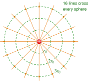
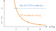
is "charge per square metre of sphere". A charge of coulombs spreads coulombs of flux over every sphere around it, and tells us how densely.
In free space, and differ only by the constant factor and carry the same information. The distinction becomes important in Section 3.4, where material media are introduced: there keeps the property we are about to discover, namely that its flux counts the (free) charge, while is modified by the material.
At from a point charge, . What is at , and what is the charge?
, so at it is . The charge is , the same from both radii: .
Flux: how much field passes through a surface
The word flux comes from the Latin for "flow". Imagine rain falling straight down, and hold a circular net (a hoop with a mesh) in it (Figure 3.2.2). How much rain passes through the net per second?
- If the net is held horizontally, facing the rain, every drop that falls on its area goes through: the amount is (rain per square metre) .
- If the net is held vertically, edge-on to the rain, the drops slide past and nothing goes through.
- If the net is tilted by an angle , look at its shadow on the ground: the drops that pass through the net are exactly those that would have fallen on its shadow. The shadow of a tilted disk is an ellipse of area , so the amount is (rain per square metre) .
The angle is measured between the rain and the normal of the net, the unit vector perpendicular to its plane. "Rain per square metre times " is precisely the scalar product of a "rain vector" with the vector .
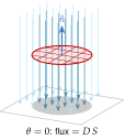
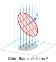
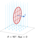
For the electric field the "rain" is the vector , and the surface need not be flat or the field uniform: we cut the surface into small elements , each practically flat, with its own normal , and add up the contributions . It is convenient to combine the area of an element and its normal into one vector, the vector surface element , familiar from the surface integrals of Section 2.3.
The electric flux through a surface is
where is the unit normal of the surface element . For a closed surface, is always taken to point outward, and is the outward flux.
The unit of flux is the coulomb: is in and in . Because the integrand is the scalar product , only the component of along the normal contributes. Figure 3.2.3 shows the three typical situations for a flat surface of area in a uniform field. When the normal is parallel to , every line crosses the surface and the flux is . When the normal is perpendicular to , the lines slide along the surface and the flux is zero. In general, with the angle between and ,
Equivalently, is the projection of the surface onto a plane perpendicular to the field, the "shadow" it casts in the stream of field lines.
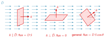
For a closed surface, such as the skin of a balloon, there is a natural choice of normal: the one pointing outward. With it, a field line that leaves the enclosed region contributes positively (), and a line that enters contributes negatively (). The outward flux is therefore a balance: what flows out minus what flows in.
Flux "how much passes through". Picture the field lines as rain: the flux through a surface counts the lines crossing it, each crossing weighted by . Through a closed surface we count outgoing lines as and incoming lines as .
A flat net of area is placed in the uniform field , with its normal at to . What is the flux through it? And through the same net turned so that its normal is at ?
. At , and : the same lines cross the net, but in the direction opposite to the chosen normal.