4.3.6 Saturation and hysteresis: the limits of the reluctance

The reluctance $Z = l / (μ S)$ presumes a constant $μ$ . For iron this is not so. Figure 4.3.8 shows the relation between $B$ and $H$ in a ferromagnetic core as the current of its winding is cycled. Starting from an unmagnetised core, $B$ follows the initial curve: it rises steeply at first, then more and more slowly, and finally the material saturates at $B_{s}$ (about $2 T$ for iron and steel), beyond which $B$ grows only as $μ_{0} H$ , as if the core were air. When $H$ is reduced again, $B$ does not retrace the initial curve but stays higher: at $H = 0$ a remanent induction $B_{r}$ is left, and a reverse field, the coercive field $- H_{c}$ , is needed to bring $B$ back to zero. Cycling $H$ between large positive and negative values traces the closed hysteresis loop. In iron, $μ = B / H$ is therefore a function of $B$ and of the previous history of the material.

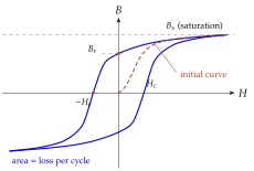
The hysteresis loop of a ferromagnetic core. From the unmagnetised state B follows the dashed initial curve up to saturation B_s. On the way back it stays above the initial curve, leaving the remanence B_r at H=0, and the coercive field H_c is needed to demagnetise it. The area of the loop is the energy lost per unit volume in each cycle. — **Figure 4.3.8.** The hysteresis loop of a ferromagnetic core. From the unmagnetised state $B$ follows the dashed initial curve up to saturation $B_{s}$ . On the way back it stays above the initial curve, leaving the remanence $B_{r}$ at $H = 0$ , and the coercive field $H_{c}$ is needed to demagnetise it. The area of the loop is the energy lost per unit volume in each cycle.

A magnetic circuit with iron in it is therefore a nonlinear circuit. The loop rule still holds, but it is written with $H$ and $B$ rather than with reluctances:

read H_{i} from the B - H curve H_{1} l_{1} + H_{2} l_{2} + \dots + \frac{B _{g}}{μ _{0}} l_{g} = N I . (4.3.21)

This is exactly how Problems 4.3.1–4.3.3 at the end of this section are solved. One never computes $μ$ . One reads $H$ off the curve of the material for the value of $B$ that each branch carries, multiplies by the length of the branch, and adds the gap term $B_{g} l_{g} / μ_{0}$ , for which the constant $μ_{0}$ is exact. Only in the home exercises and most of the further exercises, where $μ_{r}$ is given as a constant, is $Z = l / (μ S)$ used directly.

The nonlinear loop rule

Around every closed path of a circuit with iron,

iron branches \sum H_{i} l_{i} + gaps \sum \frac{B _{g}}{μ _{0}} l_{g} = \sum N I, H_{i} = H (B_{i}) from the curve, B_{i} = \frac{Φ _{i}}{S _{i}} .

In plain words

When the iron is nonlinear, forget $μ$ . Carry $B$ from branch to branch with the node rule ( $Φ$ is conserved, $B = Φ/ S$ ), look up $H$ on the curve, and add up $H l$ around the loop.

Two consequences of the loop are worth remembering.

Saturation. Beyond $B_{s}$ the core stops helping: $μ \to μ_{0}$ and the winding behaves like an air coil. A core is therefore designed to run below $B_{s}$ , and the "plateau" of the solution of Problem 4.3.1 shows what happens when a branch saturates: however hard the rest of the circuit is driven, that branch will not pass more flux.
Losses. Each cycle round the loop costs an energy per unit volume equal to the area of the loop, in $J/ m^{3}$ , so the hysteresis power is proportional to the frequency, $P_{h} \propto f$ . In a solid core the alternating flux also induces eddy currents, with a power $P_{e} \propto t^{2} f^{2} B_{m a x}^{2}$ where $t$ is the thickness of the laminations, which is why cores for alternating flux are built from thin insulated sheets.

Soft and hard magnetic materials

The shape of the loop decides what a material is good for. A soft material (narrow loop, small $H_{c}$ ) is what one wants in a core: it magnetises easily and loses little per cycle. A hard material (wide loop, large $H_{c}$ ) keeps its magnetisation when the field is removed: it is a permanent magnet. Table 4.3.2 gives typical figures. The $B_{s}$ column is the ceiling of every magnetic circuit built with that material, and the $H_{c}$ column is what the material "remembers" when the current is switched off.

Table 4.3.2. Typical soft and hard magnetic materials.

material	$B_{s}$ or $B_{r}$	$H_{c}$	typical use
80 % Ni permalloy	$0.8 T$	$\sim 1 A/m$	shields, sensor cores
Mn–Zn ferrite	$0.4$ – $0.5 T$	$10$ – $20 A/m$	switch-mode transformers
grain-oriented Si steel	$2.0 T$	$5$ – $10 A/m$	power transformers
hard ferrite (magnet)	$B_{r} \approx 0.4 T$	$\sim 250 kA/m$	small motors, loudspeakers
Nd–Fe–B (magnet)	$B_{r} \approx 1.3 T$	$\sim 1000 kA/m$	servo and traction motors

Compare a soft material with a magnet (Nd–Fe–B, $M$ against $H$ ) and see how $H_{c}$ and the loop area change by five orders of magnitude.

InteractiveLoading simulation…

Common mistake · Using a reluctance for saturated iron

Computing $Z = l / (μ_{0} μ_{r} S)$ with a handbook value of $μ_{r}$ and then finding $B = 3 T$ in a limb. Real iron saturates near $2 T$ , and a linear calculation that lands above $B_{s}$ is simply wrong: the limb would saturate, its permeability would collapse towards $μ_{0}$ , and the fluxes would be redistributed (Exercise 4.3.4 runs into exactly this). Whenever a linear answer approaches $B_{s}$ , switch to the $B$ – $H$ curve.

Quick check

A cast-steel branch $1 m$ long must carry $B = 1 T$ , for which the curve of Figure 4.3.21 gives $H = 770 A/m$ . A $1 mm$ air gap carries the same $B$ . Which takes more ampere-turns?

The steel takes $H l = 770 \times 1 = 770 At$ . The gap takes $B l_{g} / μ_{0} = 1 \times 1 0^{- 3} / (4 π \times 1 0^{- 7}) = 796 At$ . The millimetre of air costs slightly more than the metre of steel.