3.1.2 The notion of charge

Elementary charge

What is electric charge? Experimentally, it is the property that makes bodies attract or repel each other in a way that cannot be explained by their masses. Two glass rods rubbed with silk repel each other, whereas a glass rod and an amber rod rubbed with fur attract. So there are two kinds of charge, which we call positive and negative: like charges repel, unlike charges attract.

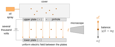
A key question is whether charge can be divided again and again without end, like a fluid, or whether it comes in lumps. R. A. Millikan's oil-drop experiments (published around 1911) answered it. The idea is simple (Figure 3.1.1):

1. Tiny oil droplets, charged by friction as they leave an atomiser, drift into the space between two horizontal metal plates.
2. A voltage of several thousand volts between the plates produces a uniform electric field, which pushes on a charged droplet with an electric force.
3. By watching a single droplet through a microscope and adjusting the field until the electric force balances the weight (or by timing the droplet's rise and fall), the charge on that droplet can be found.

Whatever droplet was chosen, the measured charge always turned out to be an integer multiple of one and the same quantity. Electric charge, therefore, cannot be made as small as desired.

The smallest quantity of charge observed in these (and all later) experiments is

called the elementary charge. Every observed free charge is a whole multiple of it, $q=\pm Ne$ with $N$ an integer. The electron carries the charge $-e$, the proton the charge $+e$, and the neutron is uncharged. An ordinary piece of matter is neutral because it contains equal numbers of electrons and protons. It becomes charged when electrons are added (negative) or removed (positive).

The masses of the three particles are very different. J. J. Thomson's cathode-ray experiments of 1897 measured the charge-to-mass ratio $e/m_e$ of the electron. Combined with Millikan's value of $e$, this gives the rest mass of the electron,

while the proton and the neutron have very similar, much larger rest masses, $m_p=1.6726\times 10^{-27}\mathrm{kg}$ and $m_n=1.6749\times 10^{-27}\mathrm{kg}$, about $1836$ and $1839$ times the electron mass. Because the electron is so light, its charge-to-mass ratio is huge, $e/m_e\approx 1.76\times 10^{11}C/kg$. This is why electrons respond so quickly to electric fields (Home exercise 3.1.3).

Charge distributions

Since $e$ is so small, a macroscopic charge of even one nanocoulomb consists of more than six billion elementary charges ($10^{-9}/1.602\times 10^{-19}\approx 6.2\times 10^9$). Nobody wants to keep track of six billion particles. When we are not interested in individual particles we therefore describe charge by a smooth density, just as we describe water by its mass density instead of counting molecules.

From many particles to a smooth density

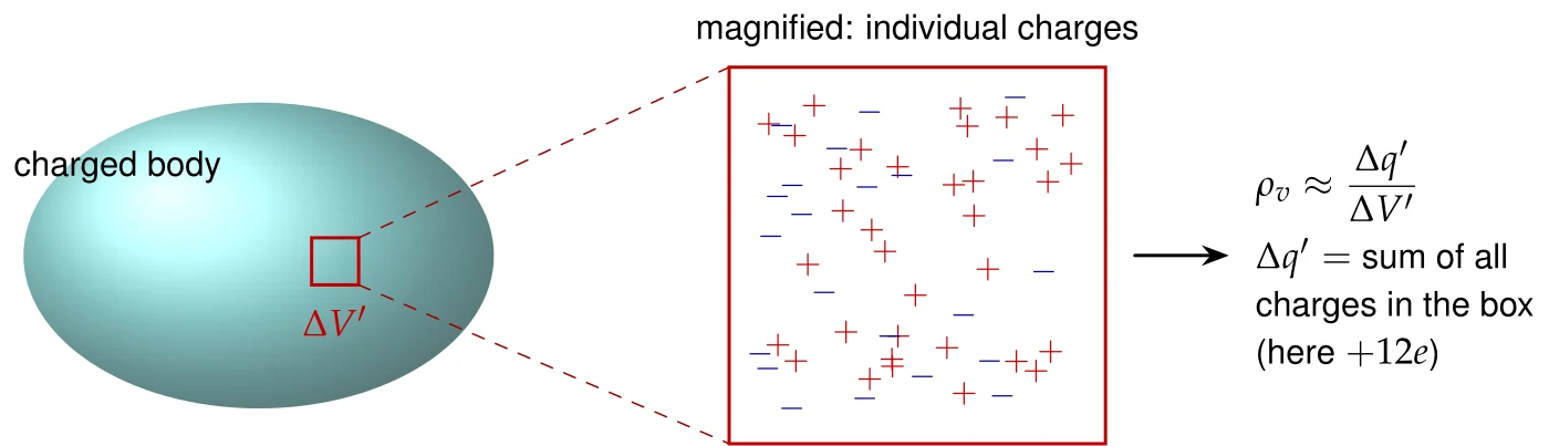
Figure 3.1.2 shows the idea. Pick a small box of volume $\Delta V^{\prime }$ inside a charged body and add up all the charges $\Delta q^{\prime }$ inside it. The box must be small compared with the body (so that the density can vary from place to place) but still large compared with atoms (so that it contains very many charges and the count does not jump about). The ratio $\Delta q^{\prime }/\Delta V^{\prime }$ is then the volume charge density at that place.

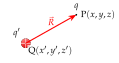
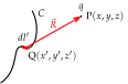
Depending on the shape of the charged object, four idealised descriptions are used (Figure 3.1.3):

• A point charge $q$ [C] is concentrated at one point. Its size is negligible compared with the distance at which we observe it.
• A line charge of density ${\rho }_L$ [C/m] is spread along a curve $C$ (a thin wire, a charged filament). An element $d{l}^{\prime }$ of the curve carries the charge $d{q}^{\prime }={\rho }_{L}d{l}^{\prime }$.
• A surface charge of density ${\rho }_S$ [C/m²] is spread over a surface $S$ (a thin sheet, the surface of a conductor). An element $d{S}^{\prime }$ carries $d{q}^{\prime }={\rho }_{S}d{S}^{\prime }$.
• A volume charge of density ${\rho }_v$ [C/m³] is spread through a region $V$ (a charged cloud, an electron beam). An element $d{V}^{\prime }$ carries $d{q}^{\prime }={\rho }_{v}d{V}^{\prime }$.

Formally,

where the limits are understood in the macroscopic sense just described ("small, but not atomic").

Primed and unprimed coordinates

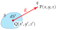
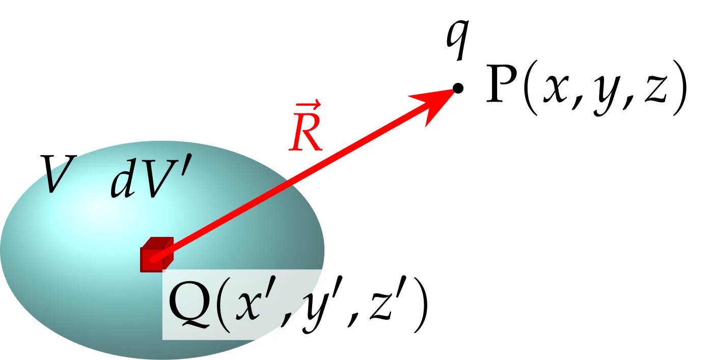
The densities may vary from point to point, so they are functions of the position of the charge. We call that position the source point $\mathrm{Q}$ and always write its coordinates with primes, $(x^{\prime },y^{\prime },z^{\prime })$. The point where we want to know the effect of the charge (the force on another charge, or later the field) is the field point $\mathrm{P}$, with unprimed coordinates $(x,y,z)$. Keeping the two sets of coordinates apart is the single most useful habit of this section.

Total charge

The total charge of a distribution is obtained by adding up the charges of all the elements:

In all three cases we can simply write $d{q}^{\prime }$ for the charge of the element, and a single formula $Q=\int d{q}^{\prime }$ covers them all. The length, area and volume elements are those of the coordinate system we use (Sections 2.3 and 2.4). For instance, a disk is described in polar coordinates with $d{S}^{\prime }={\rho }^{\prime }d{\rho }^{\prime }d{\varphi }^{\prime }$.