Exercise 3.1.6: Circular loop with a nonuniform charge

Exercise 3.1.6

About the further exercises of Section 3.1

Ten further exercises in the spirit of Problems 3.1.1 to 3.1.3 and Home exercises 3.1.1 and 3.1.2. Every one is solved with the four steps of Section 3.1.8, and the two standard integrals (3.1.30) appear again and again.

Exercise 3.1.6

Circular loop with a nonuniform charge

cf. Problem 3.1.2

The circular loop of Problem 3.1.2 (radius $b$ , in the $x y$ -plane, centred at the origin) now carries the nonuniform line charge density $ρ_{L} = ρ_{0} cos ϕ^{'}$ C/m, $ρ_{0}$ being a constant.

a) Find the total charge on the loop.

b) Find the electric field at $P (0, 0, h)$ .

Try it yourself first.

Strategy

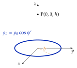
This is Problem 3.1.2 with a density that depends on $ϕ^{'}$ , so the element is $d q^{'} = ρ_{L} b d ϕ^{'}$ with $ρ_{L} = ρ_{0} cos ϕ^{'}$ . The density now multiplies the $cos ϕ^{'}$ and $sin ϕ^{'}$ in $R$ , so different angular integrals survive than for the uniform ring. Part a) is the integral of the charge element alone. In part b) we first read off from the symmetry which component survives and then integrate.

Part a): charge element and integral

The charge element is $d q^{'} = ρ_{L} d l^{'}$ with $d l^{'} = b d ϕ^{'}$ (Figure 3.1.15b), so $d q^{'} = ρ_{0} cos ϕ^{'} b d ϕ^{'}$ and the total charge is

Q = \int_{0}^{2 π} ρ_{0} cos ϕ^{'} b d ϕ^{'} = ρ_{0} b \int_{0}^{2 π} cos ϕ^{'} d ϕ^{'} .

Part a): integrate

\int_{0}^{2 π} cos ϕ^{'} d ϕ^{'} = [sin ϕ^{'}]_{0}^{2 π} = 0 - 0 = 0,

Answer

Q = 0 [C]

Check (part a)

Units: $ρ_{0} b$ is $(C/m) \cdot m = C$ . The half $x > 0$ (where $cos ϕ^{'} > 0$ ) is positively charged and the half $x < 0$ negatively, by equal amounts, as in the sketch of the problem.

Part b): symmetry

The charge is zero, but that does not make the field zero, and the symmetry has to be examined with the signs of the density in mind.

The mirror plane $y = 0$ (the $x z$ -plane) maps the loop onto itself and also the charge pattern, since $cos (- ϕ^{'}) = cos ϕ^{'}$ . It leaves P unchanged. The elements at $ϕ^{'}$ and $- ϕ^{'}$ carry the same charge and have the same $x$ - and $z$ -parts, but opposite $y$ -parts. So $E_{y} = 0$ .
The mirror plane $x = 0$ maps the loop onto itself but reverses the charge pattern, since $cos (π - ϕ^{'}) = - cos ϕ^{'}$ . The elements at $ϕ^{'}$ and $π - ϕ^{'}$ are at the same distance from P and carry opposite charges. Their $z$ -parts therefore cancel, so $E_{z} = 0$ . Their $x$ -parts add, because the $x$ -part of $R$ changes sign together with the charge.
Every element is at the same distance $R = b^{2} + h^{2}$ from P.

So $E = E_{x} a_{x}$ only, parallel to the plane of the loop. Its sign can be guessed: the positive half ( $x > 0$ ) pushes P towards $- x$ and the negative half ( $x < 0$ ) pulls it towards $- x$ as well, so $E_{x} < 0$ for $ρ_{0} > 0$ .

Part b): points and displacement vector

The source point is $Q (b cos ϕ^{'}, b sin ϕ^{'}, 0)$ and the field point is $P (0, 0, h)$ , exactly as in Problem 3.1.2:

R R = - b cos ϕ^{'} a_{x} - b sin ϕ^{'} a_{y} + h a_{z}, = b^{2} + h^{2} .

Part b): charge element and integral

With $d q^{'} = ρ_{0} cos ϕ^{'} b d ϕ^{'}$ , taking the constants out of the integral,

E (P) = \frac{1}{4 π ε _{0}} \int_{0}^{2 π} ρ_{0} cos ϕ^{'} b d ϕ^{'} \times \frac{- b cos ϕ ^{'} a _{x} - b sin ϕ ^{'} a _{y} + h a _{z}}{( b ^{2} + h ^{2} ) ^{3/2}} = \frac{ρ _{0} b}{4 π ε _{0} ( b ^{2} + h ^{2} ) ^{3/2}} {- b a_{x} \int_{0}^{2 π} cos^{2} ϕ^{'} d ϕ^{'} - b a_{y} \int_{0}^{2 π} cos ϕ^{'} sin ϕ^{'} d ϕ^{'} + h a_{z} \int_{0}^{2 π} cos ϕ^{'} d ϕ^{'}} .

Part b): integrate

Each angular integral is evaluated on its own. For the first we use $cos^{2} ϕ^{'} = \frac{1}{2} (1 + cos 2 ϕ^{'})$ , for the second $cos ϕ^{'} sin ϕ^{'} = \frac{1}{2} sin 2 ϕ^{'}$ :

\int_{0}^{2 π} cos^{2} ϕ^{'} d ϕ^{'} \int_{0}^{2 π} cos ϕ^{'} sin ϕ^{'} d ϕ^{'} \int_{0}^{2 π} cos ϕ^{'} d ϕ^{'} = [\frac{ϕ ^{'}}{2} + \frac{sin 2 ϕ ^{'}}{4}]_{0}^{2 π} = π + 0 - 0 = π, = [- \frac{cos 2 ϕ ^{'}}{4}]_{0}^{2 π} = - \frac{1}{4} + \frac{1}{4} = 0, = [sin ϕ^{'}]_{0}^{2 π} = 0.

The last two confirm $E_{y} = 0$ and $E_{z} = 0$ from the symmetry step, and only the $x$ -term survives:

E (P) = \frac{ρ _{0} b}{4 π ε _{0} ( b ^{2} + h ^{2} ) ^{3/2}} (- b π) a_{x},

that is

Answer

E (P) = - \frac{ρ _{0} b ^{2}}{4 ε _{0} ( b ^{2} + h ^{2} ) ^{3/2}} a_{x} [V/m]

Interpretation

The field is parallel to the plane of the loop and points from the positive half towards the negative half (see the sketch in the problem), in agreement with the sign predicted in the symmetry step. Its magnitude decreases monotonically with $h$ , because $(b^{2} + h^{2})^{- 3/2}$ does, so the largest value is at the centre of the loop, $E_{x} (h = 0) = - ρ_{0} / (4 ε_{0} b)$ . Although $Q = 0$ , the field is not zero: for $h ≫ b$ , $(b^{2} + h^{2})^{3/2} \to h^{3}$ and $E_{x} \to - ρ_{0} b^{2} / (4 ε_{0} h^{3})$ , which falls as $1/ h^{3}$ and not as $1/ h^{2}$ . The loop has no net charge, so it cannot look like a point charge. It looks like a dipole. Its dipole moment is

p = \oint r^{'} d q^{'} = \int_{0}^{2 π} b (cos ϕ^{'} a_{x} + sin ϕ^{'} a_{y}) ρ_{0} cos ϕ^{'} b d ϕ^{'} = ρ_{0} b^{2} (π a_{x} + 0 a_{y}) = π b^{2} ρ_{0} a_{x},

and the far field is $E ≃ - p / (4 π ε_{0} h^{3}) = - ρ_{0} b^{2} / (4 ε_{0} h^{3}) a_{x}$ , which is exactly the formula of Home exercise 3.1.4 (with $q d \to p$ ) for a point where $R \cdot d = 0$ .

Check

Units: $ρ_{0}$ is in C/m, so $ρ_{0} b^{2} / [ε_{0} (b^{2} + h^{2})^{3/2}]$ is $(C/m) m^{2} / (F/m \cdot m^{3}) = V/m$ . Direction: from the positive half to the negative half, parallel to the loop, and flipping sign if $ρ_{0}$ changes sign. Far-field limit: the dipole field, as shown above.