Home exercise 3.1.2: Annular arc with nonuniform charge

Home exercise 3.1.2

Annular arc with nonuniform charge

As shown in the figure, there is an annular arc on the $x y$ -plane described by

a \leq ρ \leq b, 0 \leq ϕ \leq π /2, z = 0.

On this surface a nonuniform surface charge density is given as

ρ_{S} (ρ^{'}, ϕ^{'}) = \frac{2 cos ϕ ^{'}}{ρ ^{'}} C/ m^{2} .

a) Find the total charge on the annular arc.

b) Using Coulomb's law, express the electric field due to this charge distribution at a point $h$ on the $z$ -axis.

Try it yourself first.

Strategy

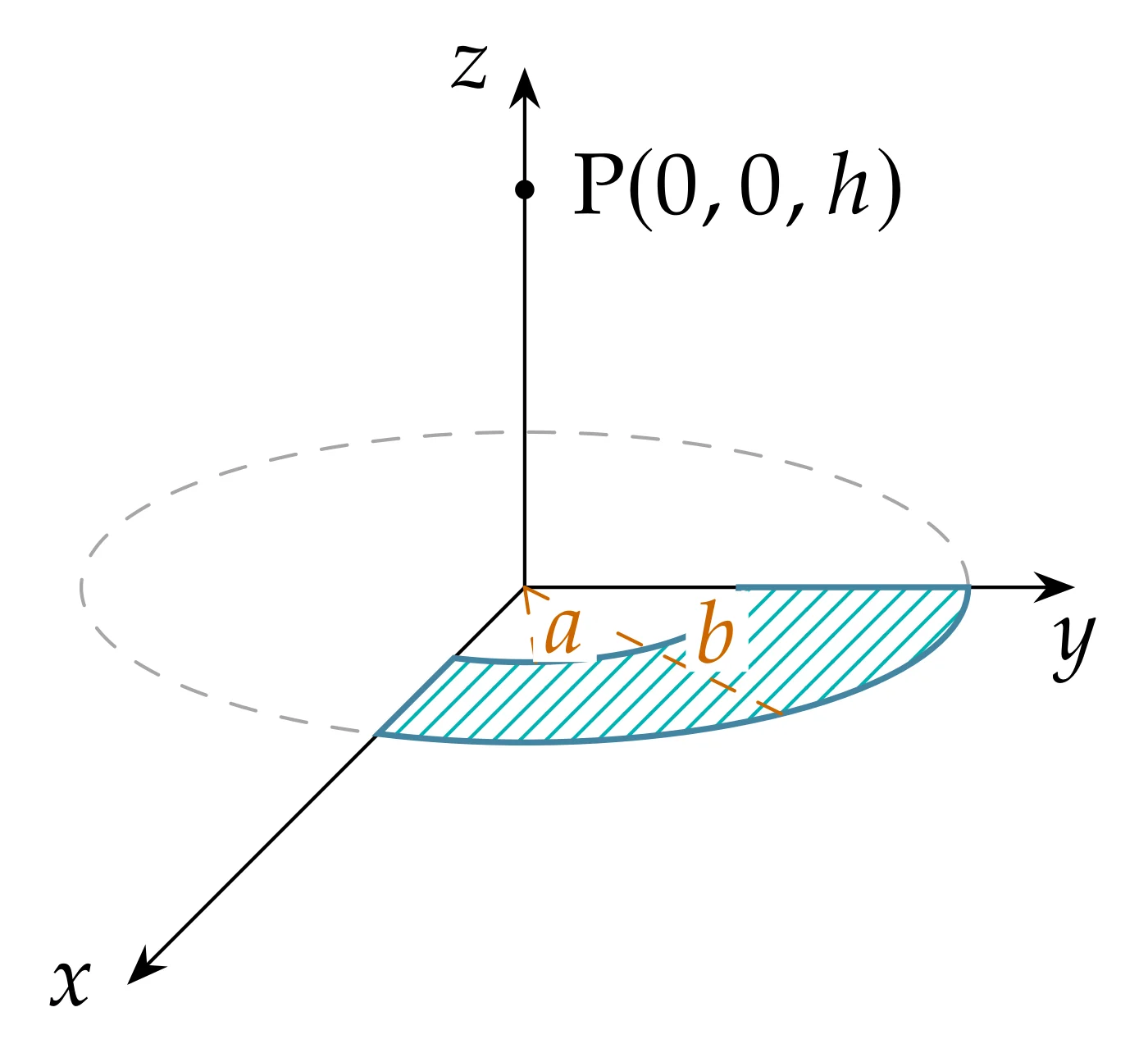
Part a) is a surface integral of $ρ_{S}$ with $d S^{'} = ρ^{'} d ρ^{'} d ϕ^{'}$ . Part b) is the recipe of Problem 3.1.3 with a surface source, but the charge occupies only a quarter of an annulus and depends on $ϕ^{'}$ . No symmetric partner cancels the horizontal components, so all three components must be computed. Because the density is a product of a function of $ρ^{'}$ and a function of $ϕ^{'}$ , the double integrals separate into an angular and a radial factor, and the radial ones are the standard integrals (3.1.30).

Part a): total charge

The total charge is the integral of the surface density over the surface, $Q = \int_{S} ρ_{S} d S^{'}$ . On the annular arc the area element is $d S^{'} = ρ^{'} d ϕ^{'} d ρ^{'}$ , and we do not forget the factor $ρ^{'}$ (Figure 3.1.15c). Inserting $ρ_{S} = 2 cos ϕ^{'} / ρ^{'}$ and the limits $a \leq ρ^{'} \leq b$ , $0 \leq ϕ^{'} \leq π /2$ ,

Q = \int_{ρ^{'} = a}^{b} \int_{ϕ^{'} = 0}^{π /2} \frac{2 cos ϕ ^{'}}{ρ ^{'}} ρ^{'} d ϕ^{'} d ρ^{'} = 2 \int_{a}^{b} \int_{0}^{π /2} cos ϕ^{'} d ϕ^{'} d ρ^{'} .

The factor $ρ^{'}$ of the area element cancels the $1/ ρ^{'}$ of the density. What is left no longer depends on $ρ^{'}$ in the integrand, so the two integrals can be done one after the other:

\int_{0}^{π /2} cos ϕ^{'} d ϕ^{'} Q = [sin ϕ^{'}]_{0}^{π /2} = 1 - 0 = 1, = 2 \int_{a}^{b} 1 d ρ^{'} = 2 [ρ^{'}]_{a}^{b} = 2 (b - a) .

Answer

Q = 2 (b - a) [C]

The constant $2$ in $ρ_{S}$ carries the unit C/m, because $ρ_{S}$ is in C/m² and $cos ϕ^{'} / ρ^{'}$ is in 1/m. Hence $2 (b - a)$ is in coulombs. Note that the charge does not depend on the order of the integrals and grows linearly with the radial width $b - a$ .

Part b): symmetry

We now look for the electric field at $P (0, 0, h)$ on the $z$ -axis, and here symmetry helps much less than for the disk of Problem 3.1.3.

The charge fills only the first quadrant, so a rotation about the $z$ -axis does not map the source onto itself, and the argument of Problem 3.1.3 (the $ϕ^{'}$ -integral of $cos ϕ^{'}$ and $sin ϕ^{'}$ over a full turn) is not available.
The density $2 cos ϕ^{'} / ρ^{'}$ is not even symmetric about the plane $ϕ^{'} = π /4$ , because $cos ϕ^{'} \neq = cos (π /2 - ϕ^{'}) = sin ϕ^{'}$ . Hence there is no mirror partner either.
So all three components $E_{x}$ , $E_{y}$ , $E_{z}$ can be different from zero. Their signs follow from the geometry: all the charge lies at $x^{'} \geq 0$ , $y^{'} \geq 0$ and $z^{'} = 0$ , so for a positive charge it pushes P to $- x$ , to $- y$ and up along $+ z$ .

What does survive is the separation of the integrals: $ρ_{S}$ is a product $f (ρ^{'}) g (ϕ^{'})$ , and every component of $R / R^{3}$ is a product of a function of $ρ^{'}$ and a function of $ϕ^{'}$ . This is what makes the calculation manageable.

Part b): points and displacement vector

The source point is $Q (x^{'}, y^{'}, 0)$ with $x^{'} = ρ^{'} cos ϕ^{'}$ , $y^{'} = ρ^{'} sin ϕ^{'}$ , $a \leq ρ^{'} \leq b$ , $0 \leq ϕ^{'} \leq π /2$ , and the field point is $P (0, 0, h)$ . Then

R R = (0 - x^{'}) a_{x} + (0 - y^{'}) a_{y} + (h - 0) a_{z} = - ρ^{'} cos ϕ^{'} a_{x} - ρ^{'} sin ϕ^{'} a_{y} + h a_{z}, = (ρ^{'})^{2} cos^{2} ϕ^{'} + (ρ^{'})^{2} sin^{2} ϕ^{'} + h^{2} = (ρ^{'})^{2} + h^{2} .

These are the vectors of Problem 3.1.3, and $R$ depends on $ρ^{'}$ only.

Part b): charge element and integral

The charge element is $d q^{'} = ρ_{S} d S^{'} = \frac{2 cos ϕ ^{'}}{ρ ^{'}} ρ^{'} d ϕ^{'} d ρ^{'} = 2 cos ϕ^{'} d ϕ^{'} d ρ^{'}$ , so the electric field at P is

E (P) = \frac{1}{4 π ε _{0}} \int_{ρ^{'} = a}^{b} \int_{ϕ^{'} = 0}^{π /2} 2 cos ϕ^{'} d ϕ^{'} d ρ^{'} \times \frac{- ρ ^{'} cos ϕ ^{'} a _{x} - ρ ^{'} sin ϕ ^{'} a _{y} + h a _{z}}{[ ( ρ ^{'} ) ^{2} + h ^{2} ] ^{3/2}} = \frac{1}{2 π ε _{0}} \int_{a}^{b} \int_{0}^{π /2} cos ϕ^{'} d ϕ^{'} d ρ^{'} \times \frac{- ρ ^{'} cos ϕ ^{'} a _{x} - ρ ^{'} sin ϕ ^{'} a _{y} + h a _{z}}{[ ( ρ ^{'} ) ^{2} + h ^{2} ] ^{3/2}} .

Now we separate the components. The unit vectors are constant, and the denominator contains only $ρ^{'}$ :

E (P) = \frac{1}{2 π ε _{0}} \int_{a}^{b} \frac{ρ ^{'}}{[ ( ρ ^{'} ) ^{2} + h ^{2} ] ^{3/2}} \times {- a_{x} \int_{0}^{π /2} cos^{2} ϕ^{'} d ϕ^{'} - a_{y} \int_{0}^{π /2} cos ϕ^{'} sin ϕ^{'} d ϕ^{'}} d ρ^{'} + \frac{h a _{z}}{2 π ε _{0}} \int_{a}^{b} \frac{1}{[ ( ρ ^{'} ) ^{2} + h ^{2} ] ^{3/2}} \times {\int_{0}^{π /2} cos ϕ^{'} d ϕ^{'}} d ρ^{'} .

Part b): integrate

Angular integrals. Each is done on its own line. For the first we use the identity $cos^{2} ϕ^{'} = \frac{1}{2} (1 + cos 2 ϕ^{'})$ :

\int_{0}^{π /2} cos^{2} ϕ^{'} d ϕ^{'} = \frac{1}{2} \int_{0}^{π /2} [1 + cos 2 ϕ^{'}] d ϕ^{'} = [\frac{ϕ ^{'}}{2} + \frac{1}{4} sin 2 ϕ^{'}]_{0}^{π /2} = \frac{π}{4} + 0 - 0 = \frac{π}{4}, \int_{0}^{π /2} cos ϕ^{'} sin ϕ^{'} d ϕ^{'} = \frac{1}{2} \int_{0}^{π /2} sin 2 ϕ^{'} d ϕ^{'} = [- \frac{1}{4} cos 2 ϕ^{'}]_{0}^{π /2} = \frac{1}{4} + \frac{1}{4} = \frac{1}{2}, \int_{0}^{π /2} cos ϕ^{'} d ϕ^{'} = [sin ϕ^{'}]_{0}^{π /2} = 1.

Inserting them,

E (P) = \frac{1}{2 π ε _{0}} (- \frac{π}{4} a_{x} - \frac{1}{2} a_{y}) \times \int_{a}^{b} \frac{ρ ^{'} d ρ ^{'}}{[ ( ρ ^{'} ) ^{2} + h ^{2} ] ^{3/2}} + \frac{h a _{z}}{2 π ε _{0}} \int_{a}^{b} \frac{d ρ ^{'}}{[ ( ρ ^{'} ) ^{2} + h ^{2} ] ^{3/2}} .

Radial integrals. They are exactly the two standard integrals (3.1.30), with $s = ρ^{'}$ and the same constant $h$ :

\int_{a}^{b} \frac{ρ ^{'} d ρ ^{'}}{[ ( ρ ^{'} ) ^{2} + h ^{2} ] ^{3/2}} = [- \frac{1}{( ρ ^{'} ) ^{2} + h ^{2}}]_{a}^{b} = - \frac{1}{b ^{2} + h ^{2}} + \frac{1}{a ^{2} + h ^{2}}, \int_{a}^{b} \frac{d ρ ^{'}}{[ ( ρ ^{'} ) ^{2} + h ^{2} ] ^{3/2}} = [\frac{ρ ^{'}}{h ^{2} ( ρ ^{'} ) ^{2} + h ^{2}}]_{a}^{b} = \frac{b}{h ^{2} b ^{2} + h ^{2}} - \frac{a}{h ^{2} a ^{2} + h ^{2}} .

In the $z$ -term the factor $h$ in front cancels one power of $h$ of the second integral, since $h \cdot \frac{1}{h ^{2}} = \frac{1}{h}$ . Collecting the three components,

Answer

E (P) = \frac{1}{2 π ε _{0}} (- \frac{π}{4} a_{x} - \frac{1}{2} a_{y}) \times [\frac{1}{a ^{2} + h ^{2}} - \frac{1}{b ^{2} + h ^{2}}] + a_{z} \frac{1}{2 π ε _{0}} \times [\frac{b}{h b ^{2} + h ^{2}} - \frac{a}{h a ^{2} + h ^{2}}] [V/m]

Interpretation and limits

The $x$ -component is larger in magnitude than the $y$ -component, in the ratio $π /4 : 1/2 = π /2$ , because $cos ϕ^{'}$ puts more charge near the $x$ -axis. Both are negative because the (positive) charge lies in the first quadrant and pushes P away from it.
$h \to 0$ (P at the origin, the corner of the quarter annulus): the bracket of $E_{z}$ behaves as $\frac{h}{2} (\frac{1}{a ^{2}} - \frac{1}{b ^{2}})$ , so $E_{z} \to 0$ , while the horizontal part tends to

$\frac{1}{2 π ε _{0}} (- \frac{π}{4} a_{x} - \frac{1}{2} a_{y}) (\frac{1}{a} - \frac{1}{b}) .$

In the plane of the charge the field is purely horizontal.
$h ≫ b$ : the bracket of $E_{z}$ becomes $(b - a) / h^{2}$ and, since $\frac{1}{a ^{2} + h ^{2}} - \frac{1}{b ^{2} + h ^{2}} ≃ \frac{b ^{2} - a ^{2}}{2 h ^{3}}$ ,

$E_{z} ≃ \frac{1}{2 π ε _{0} h} [\frac{b}{h} - \frac{a}{h}] = \frac{2 ( b - a )}{4 π ε _{0} h ^{2}} = \frac{Q}{4 π ε _{0} h ^{2}},$

the field of the total charge found in part a), while the horizontal components fall off faster, as $1/ h^{3}$ .

Check

Units: the constant $2$ in $ρ_{S}$ is in C/m, so $2/ (ε_{0} \cdot length)$ is $(C/m) / (F/m \cdot m) = V/m$ in every term, and every bracket is in 1/m. Direction: away from the charge, as found in the symmetry step of part b). Far field: the point-charge field of $Q = 2 (b - a)$ , the total charge of part a).