Electromagnetic Fields and Waves: Notes, Solved Problems and Interactive Lab

Problem 3.1.1

Interactive: Finite Line Charge

Problem 3.1.1

Infinitely long line source

Find the electric field at a normal distance $ρ$ from an infinitely long line charge with a uniform charge density $ρ_{L}$ .

Source: D. K. Cheng, Field and Wave Electromagnetics, 2nd ed., Example 3-4.

Try it yourself first.

Strategy

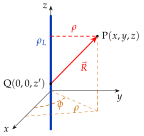
Use the recipe of Section 3.1.8 with a line source, $d q^{'} = ρ_{L} d z^{'}$ . Before integrating, let the symmetry of the infinite line tell us which components can survive. Then only one scalar integral is left, and it is one of the standard integrals (3.1.30).

Symmetry

Half of this problem is settled before any integral is written, just by looking at the geometry (Figure 3.1.23). We place the line on the $z$ -axis.

Sliding the whole line along $z$ changes nothing, so $E$ cannot depend on $z$ .
Rotating it about the $z$ -axis changes nothing, so $E$ cannot depend on $ϕ$ , and it cannot have a $ϕ$ -component either (a rotation by $18 0^{\circ}$ about the perpendicular from P to the line maps the line onto itself but reverses any $ϕ$ -component).
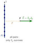
Every element $d l^{'}$ at height $z + s$ above P is matched by an element at height $z - s$ below it. Their contributions have equal and opposite $z$ -components and equal $ρ$ -components. So $E$ has no $z$ -component.

What is left is a single unknown function of a single variable, $E = E_{ρ} (ρ) a_{ρ}$ , and the integral only has to produce one number for each $ρ$ . The habit worth building is to read the symmetry off the geometry first, then integrate only what is genuinely unknown.

Problem 3.1.1, the symmetric-partner argument in three steps. (a) A single element dl' above P produces a field d\vec E_1 that points away from it, with a radial part dE_\rho and a z-part dE_z. (b) The element at the same distance below P (its mirror partner) gives the same radial part and the opposite z-part. (c) The whole line consists of such pairs, so only the radial component survives. — **Figure 3.1.23.** Problem 3.1.1, the symmetric-partner argument in three steps. (a) A single element $d l^{'}$ above P produces a field $d E_{1}$ that points away from it, with a radial part $d E_{ρ}$ and a $z$ -part $d E_{z}$ . (b) The element at the same distance below P (its mirror partner) gives the same radial part and the opposite $z$ -part. (c) The whole line consists of such pairs, so only the radial component survives.

Points and displacement vector

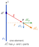
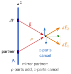
The source point is $Q (0, 0, z^{'})$ , $- \infty < z^{'} < \infty$ , and the field point is $P (x, y, z)$ . The displacement vector and its magnitude are

R R = (x - 0) a_{x} + (y - 0) a_{y} + (z - z^{'}) a_{z} = x a_{x} + y a_{y} + (z - z^{'}) a_{z}, = x^{2} + y^{2} + (z - z^{'})^{2} = ρ^{2} + (z - z^{'})^{2},

where $ρ = x^{2} + y^{2}$ is the normal distance from P to the line.

Charge element and integral

On the straight line $d l^{'} = d z^{'}$ , so $d q^{'} = ρ_{L} d z^{'}$ and the electric field at P is

E (P) = \frac{1}{4 π ε _{0}} \int_{z^{'} = - \infty}^{\infty} ρ_{L} d z^{'} \times \frac{x a _{x} + y a _{y} + ( z - z ^{'} ) a _{z}}{[ ρ ^{2} + ( z - z ^{'} ) ^{2} ] ^{3/2}},

or, separating the components (and writing $(z - z^{'}) = - (z^{'} - z)$ ),

E (P) = \frac{ρ _{L}}{4 π ε _{0}} {(x a_{x} + y a_{y}) \int_{- \infty}^{\infty} \frac{d z ^{'}}{[ ρ ^{2} + ( z ^{'} - z ) ^{2} ] ^{3/2}} - a_{z} \int_{- \infty}^{\infty} \frac{( z ^{'} - z ) d z ^{'}}{[ ρ ^{2} + ( z ^{'} - z ) ^{2} ] ^{3/2}}} .

Note that $x$ , $y$ and $z$ belong to the fixed field point: during the integration over $z^{'}$ they are constants, which is why $x a_{x} + y a_{y}$ could be taken outside.

Integrate

The first integral is evaluated with the substitution $z^{'} - z = ρ tan θ$ , $d z^{'} = ρ d θ / cos^{2} θ$ , $ρ^{2} + (z^{'} - z)^{2} = ρ^{2} / cos^{2} θ$ :

\int \frac{d z ^{'}}{[ ρ ^{2} + ( z ^{'} - z ) ^{2} ] ^{3/2}} = \int \frac{ρ / cos ^{2} θ}{ρ ^{3} / cos ^{3} θ} d θ = \frac{1}{ρ ^{2}} \int cos θ d θ = \frac{sin θ}{ρ ^{2}},

\int_{- \infty}^{\infty} \frac{d z ^{'}}{[ ρ ^{2} + ( z ^{'} - z ) ^{2} ] ^{3/2}} = \frac{1}{ρ ^{2}} \frac{z ^{'} - z}{ρ ^{2} + ( z ^{'} - z ) ^{2}}_{z^{'} = - \infty}^{\infty} = \frac{1}{ρ ^{2}} [1 - (- 1)] = \frac{2}{ρ ^{2}} .

The second one is evaluated with $t = (z^{'} - z)^{2} + ρ^{2}$ , $d t = 2 (z^{'} - z) d z^{'}$ :

\int \frac{( z ^{'} - z ) d z ^{'}}{[ ρ ^{2} + ( z ^{'} - z ) ^{2} ] ^{3/2}} = \frac{1}{2} \int \frac{d t}{t ^{3/2}} = - \frac{1}{t ^{1/2}} = - \frac{1}{ρ ^{2} + ( z ^{'} - z ) ^{2}}_{z^{'} = - \infty}^{\infty} = 0 - 0 = 0,

exactly as the symmetry argument predicted (the integrand is odd about $z^{'} = z$ ). Finally, since $x a_{x} + y a_{y} = ρ cos ϕ a_{x} + ρ sin ϕ a_{y} = ρ a_{ρ}$ ,

E (P) = \frac{ρ _{L}}{4 π ε _{0}} ρ a_{ρ} \frac{2}{ρ ^{2}},

that is

Answer

E (P) = \frac{ρ _{L}}{2 π ε _{0} ρ} a_{ρ} [V/m]

Interpretation

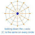
The field is radial, outward for $ρ_{L} > 0$ , and the same on every circle around the line (Figure 3.1.24, right). It decreases as $1/ ρ$ , not as $1/ ρ^{2}$ : doubling the distance halves the field, whereas a point charge would give a quarter (Figure 3.1.24, left). The reason is that, as we move away, the contribution of each element weakens as $1/ R^{2}$ but we "see" an ever longer piece of the line at nearly the same distance, and the two effects partly compensate. A dimensional argument confirms the form of the result: the only length in the problem is $ρ$ , and $ρ_{L} / ε_{0}$ has the unit of volts, so the field can only be a number times $ρ_{L} / (ε_{0} ρ)$ .

Problem 3.1.1. Left: the 1/\rho field of a line charge compared with the 1/\rho^2 field of a point charge. Right: the field lines, seen along the line, are radial. — **Figure 3.1.24.** Problem 3.1.1. Left: the $1/ ρ$ field of a line charge compared with the $1/ ρ^{2}$ field of a point charge. Right: the field lines, seen along the line, are radial.

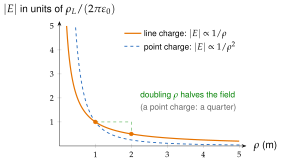
To get a feeling for the numbers, a line carrying $ρ_{L} = 1 nC/m$ in air produces $ρ_{L} / (2 π ε_{0} ρ) = 18.00/ ρ V/m$ , i.e. $1.80 kV/m$ at $1 cm$ , $180 V/m$ at $10 cm$ , $18.0 V/m$ at $1 m$ and $1.80 V/m$ at $10 m$ : ten times further out, ten times weaker.

How long must a line be to count as infinite?

Most of the field comes from the part of the line close to P. Using the antiderivative found above, the section $∣ z^{'} - z ∣ \leq ρ$ alone contributes $\int_{- ρ}^{ρ} ρ d z^{'} / (ρ^{2} + z^{'2})^{3/2} = 2 / ρ$ , i.e. $1/ 2 \approx 71 %$ of the total $2/ ρ$ . A finite wire of length $2 L$ therefore behaves like an infinite one at points near its middle as long as $ρ ≪ L$ . Home exercise 3.1.1 gives the exact correction factor $L / L^{2} + ρ^{2}$ .

Check

Units: $ρ_{L} / (ε_{0} ρ)$ is $(C/m) / (F/m \cdot m) = V/m$ . Direction: away from a positive line, as for every element. Symmetry: no $z$ - or $ϕ$ -component, as predicted in Step 1.

Move the field point and change the length of the line: near the middle of a long line the field follows the infinite-line value $ρ_{L} / (2 π ε_{0} ρ)$ , and it departs from it once $ρ$ becomes comparable with the length.

InteractiveLoading simulation…

Problem 3.1.1: Infinitely long line source