Electromagnetic Fields and Waves: Notes, Solved Problems and Interactive Lab

Point charges

Since the force of a set of charges is the sum of the individual forces and every force is $q$ times a field, the fields themselves add. For $N$ point charges $q_{k}$ at $r_{k}$ (Figure 3.1.14 with the field point P in place of $q$ ), dividing (3.1.15) by $q$ :

Superposition of electric fields

E a_{R_{k}} = \frac{1}{4 π ε _{0}} k = 1 \sum N \frac{q _{k}}{( R _{k} ) ^{2}} a_{R_{k}} = \frac{1}{4 π ε _{0}} k = 1 \sum N \frac{q _{k}}{( R _{k} ) ^{3}} R_{k}, = \frac{R _{k}}{R _{k}}, R_{k} = r - r_{k} . (3.1.25)

In the numerical illustration of Section 3.1.5, for example, the field at P is $E = F / q = (1.08 a_{x} + 0.81 a_{y}) nN /1 nC = (1.08 a_{x} + 0.81 a_{y}) V/m$ .

Field-line pictures of two charges

Figure 3.1.21 shows the result for two charges of equal magnitude. The field lines were computed from (3.1.25) and (3.1.24) by a short program that starts at a charge and keeps taking small steps in the direction of $E$ . They look entirely different for unlike and for like charges, although each picture is just the vector sum of two radial patterns of Figure 3.1.20.

(b) +q and +q. Computed field lines of two point charges a distance 2 apart (16 lines leave each positive charge at equal angles). (a) Unlike charges: the lines leave +q and end on -q, and far away the pattern is that of the dipole of Home exercise 3.1.4. (b) Like charges: the lines of the two charges bend away from each other, and midway between the charges (open circle) there is a point where \vec E=0. — **Figure 3.1.21.** (b) $+ q$ and $+ q$ . Computed field lines of two point charges a distance $2$ apart (16 lines leave each positive charge at equal angles). (a) Unlike charges: the lines leave $+ q$ and end on $- q$ , and far away the pattern is that of the dipole of Home exercise 3.1.4. (b) Like charges: the lines of the two charges bend away from each other, and midway between the charges (open circle) there is a point where $E = 0$ .

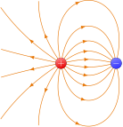
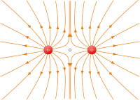
Unequal charges

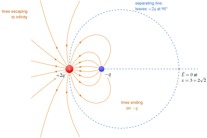
When the charges are unequal, not every line can end on the smaller one. Figure 3.1.22 shows $+ 2 q$ and $- q$ . Of the $16$ lines that leave $+ 2 q$ , exactly $8$ end on $- q$ , while the other $8$ go off to infinity, as if they came from the net charge $+ q$ seen from far away. The two families are separated by a special line (dashed), which leaves $+ 2 q$ at exactly $9 0^{\circ}$ to the axis and runs into a point where $E = 0$ . On the axis beyond $- q$ that null point is where the two fields cancel:

⟹ ⟹ \frac{2 q}{( x + 1 ) ^{2}} = \frac{q}{( x - 1 ) ^{2}} x + 1 = 2 (x - 1) x = \frac{2 + 1}{2 - 1} = 3 + 22 \approx 5.83,

in units of half the spacing between the charges.

Computed field lines of the unequal pair +2q (at x=-1) and -q (at x=+1). Lines that leave +2q within 90^\circ of the direction towards -q end on -q (8 of 16, matching the ratio of the charges), and the others escape to infinity. The dashed separating line runs into the null point x=3+2\sqrt2\approx5.83 on the axis, where \vec E=0. — **Figure 3.1.22.** Computed field lines of the unequal pair $+ 2 q$ (at $x = - 1$ ) and $- q$ (at $x = + 1$ ). Lines that leave $+ 2 q$ within $9 0^{\circ}$ of the direction towards $- q$ end on $- q$ (8 of 16, matching the ratio of the charges), and the others escape to infinity. The dashed separating line runs into the null point $x = 3 + 22 \approx 5.83$ on the axis, where $E = 0$ .

Quick check

For $+ q$ and $+ q$ (Figure 3.1.21b), where is $E = 0$ ? For $+ q$ and $- q$ , is there any point at a finite distance where $E = 0$ ?

Like charges: exactly midway, where the two equal fields point in opposite directions. Unlike charges: no. A zero needs two fields of equal size pointing in opposite directions. Equal size means equal distances from the two charges, i.e. a point of the perpendicular bisector. But there the fields of $+ q$ and $- q$ both have a component along the axis towards $- q$ , and these add instead of cancelling.

Continuous distributions

For continuous distributions the force integrals (3.1.17) to (3.1.19), divided by $q$ , give the fields of the three types of source:

Electric field of continuous charge distributions

Line charge:

E = \frac{1}{4 π ε _{0}} \int_{C} \frac{ρ _{L}}{R ^{2}} a_{R} d l^{'} = \frac{1}{4 π ε _{0}} \int_{C} ρ_{L} (x^{'}, y^{'}, z^{'}) \frac{R}{R ^{3}} d l^{'}, (3.1.26)

surface charge:

E = \frac{1}{4 π ε _{0}} \iint_{S} \frac{ρ _{S}}{R ^{2}} a_{R} d S^{'} = \frac{1}{4 π ε _{0}} \iint_{S} ρ_{S} (x^{'}, y^{'}, z^{'}) \frac{R}{R ^{3}} d S^{'}, (3.1.27)

volume charge:

E = \frac{1}{4 π ε _{0}} ∭_{V} \frac{ρ _{v}}{R ^{2}} a_{R} d V^{'} = \frac{1}{4 π ε _{0}} ∭_{V} ρ_{v} (x^{'}, y^{'}, z^{'}) \frac{R}{R ^{3}} d V^{'} . (3.1.28)

All three, and the sum (3.1.25) as well, are contained in the single compact formula

E (P) d q^{'} = \frac{1}{4 π ε _{0}} \int \frac{R}{R ^{3}} d q^{'}, = ρ_{L} d l^{'}, ρ_{S} d S^{'}, ρ_{v} d V^{'}, (3.1.29)

which is nothing but Coulomb's law for the element $d q^{'}$ , summed over the source.

In plain words

To find the field of any charged object: cut it into tiny pieces, treat each piece as a point charge, write its field with the vector $R$ from the piece to P, and add all these little fields, component by component.

Watch Eq. (3.1.29) being built: the line charge is replaced by $N$ point charges, and as $N$ grows the summed field at P settles on the value of the integral. The same construction for a ring or a disk converges to the results of Problems 3.1.2 and 3.1.3.

InteractiveLoading simulation…

Common mistake · Mixing up

x^{'}, y^{'}

and

x, y

Inside the integral only the primed (source) coordinates vary. If a field-point coordinate such as $x$ appears under $\int d x^{'}$ , it is a constant there. If a primed coordinate survives in the final answer, something went wrong. And the field point must not be moved onto the source: P is fixed while Q runs over the whole distribution.

A recipe for field calculations

All problems at the end of this section are solved with the same four steps.

Recipe · Computing

E

of a continuous distribution

Draw and name the points. Sketch the source and mark a general source point $Q$ (primed coordinates, parametrised so that they run over the whole source) and the field point $P$ (unprimed, fixed).
Build $R$ . Form $R = r - r^{'}$ (field point minus source point) in Cartesian components, and its length $R = ∣ R ∣$ .
Write the charge element. $d q^{'} = ρ_{L} d l^{'}$ or $ρ_{S} d S^{'}$ or $ρ_{v} d V^{'}$ , with the correct length, area or volume element of the coordinate system used (for instance $d l^{'} = b d ϕ^{'}$ on a circle of radius $b$ , $d S^{'} = ρ^{'} d ρ^{'} d ϕ^{'}$ on a disk), and set up (3.1.29).
Use symmetry, then integrate. Decide which components must vanish (look for symmetric partners), integrate the others component by component in $a_{x}, a_{y}, a_{z}$ , and check: units, direction, and limiting cases (very near, and very far, where the answer must become the field of a point charge carrying the total charge).

Two standard integrals

Two integrals appear again and again. With $s$ the integration variable and $h > 0$ a constant,

\int \frac{s d s}{( s ^{2} + h ^{2} ) ^{3/2}} \int \frac{d s}{( s ^{2} + h ^{2} ) ^{3/2}} = - \frac{1}{s ^{2} + h ^{2}}, = \frac{s}{h ^{2} s ^{2} + h ^{2}} . (3.1.30)

The first follows from the substitution $t = s^{2} + h^{2}$ , $d t = 2 s d s$ : $\int s d s / (s^{2} + h^{2})^{3/2} = \frac{1}{2} \int t^{- 3/2} d t = - t^{- 1/2}$ .
The second follows from $s = h tan θ$ , which gives $d s = h d θ / cos^{2} θ$ and $s^{2} + h^{2} = h^{2} / cos^{2} θ$ , so that the integrand becomes $cos θ d θ / h^{2}$ . The integral is $sin θ / h^{2}$ , and since $sin θ = s / s^{2} + h^{2}$ it equals $s / (h^{2} s^{2} + h^{2})$ .

Both are easily checked by differentiation.