Exercise 3.1.2: Finite line charge, field on its own axis

About the further exercises of Section 3.1

Ten further exercises in the spirit of Problems 3.1.1 to 3.1.3 and Home exercises 3.1.1 and 3.1.2. Every one is solved with the four steps of Section 3.1.8, and the two standard integrals (3.1.30) appear again and again.

Exercise 3.1.2

Finite line charge, field on its own axis

cf. Home exercise 3.1.1

A line charge of uniform density $ρ_{L}$ lies on the $z$ -axis from $z = - L$ to $z = + L$ . Find the electric field at the point $P (0, 0, h)$ on the same axis, with $h > L$ .

Source: D. K. Cheng, Field and Wave Electromagnetics, 2nd ed., Example 3-10.

Try it yourself first.

Strategy

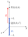
P lies on the line's own axis, so $R$ is parallel to $a_{z}$ for every element. The vector integral reduces to one elementary scalar integral, and no component has to be discarded. We follow the four steps of the recipe nevertheless, because the steps are the same for every source.

Symmetry

Here the symmetry argument is of a different kind than for the ring or the disk.

Both the line and the point P lie on the $z$ -axis, so rotating everything about the $z$ -axis changes nothing. The field at P cannot single out a horizontal direction, so it must point along $z$ .
More directly, every element lies on the axis and $R$ is parallel to it, so every contribution $d E$ already points along $\pm a_{z}$ and there is no horizontal part to cancel.
Since $h > L$ , P lies beyond the upper end of the line, so all elements lie below P. Their contributions all point upwards and add. There is no cancellation at all, whereas on the bisector of Home exercise 3.1.1 the horizontal parts cancelled in pairs.

So $E = E_{z} a_{z}$ , and one scalar integral is left.

Points and displacement vector

The source point is $Q (0, 0, z^{'})$ with $- L \leq z^{'} \leq L$ , and the field point is $P (0, 0, h)$ . Then

R = (0 - 0) a_{x} + (0 - 0) a_{y} + (h - z^{'}) a_{z} = (h - z^{'}) a_{z} .

Since $h > L \geq z^{'}$ , the number $h - z^{'}$ is positive for every element, so the magnitude is

R = ∣ h - z^{'} ∣ = h - z^{'} .

(Without the condition $h > L$ the absolute value would matter, and for $∣ h ∣ < L$ the point P would lie on the charge itself, where the field is not defined.)

Charge element and integral

On the straight line $d l^{'} = d z^{'}$ , so $d q^{'} = ρ_{L} d z^{'}$ and the electric field at P is

E (P) = \frac{ρ _{L}}{4 π ε _{0}} \int_{z^{'} = - L}^{L} \frac{( h - z ^{'} ) a _{z}}{( h - z ^{'} ) ^{3}} d z^{'} = \frac{ρ _{L}}{4 π ε _{0}} a_{z} \int_{- L}^{L} \frac{d z ^{'}}{( h - z ^{'} ) ^{2}},

because $R / R^{3} = (h - z^{'}) a_{z} / (h - z^{'})^{3} = a_{z} / (h - z^{'})^{2}$ .

Integrate

Neither of the standard integrals (3.1.30) is needed, since $R = h - z^{'}$ is linear in $z^{'}$ . We use the substitution $u = h - z^{'}$ , $d u = - d z^{'}$ . The limits change to $u = h + L$ at $z^{'} = - L$ and $u = h - L$ at $z^{'} = L$ :

\int_{- L}^{L} \frac{d z ^{'}}{( h - z ^{'} ) ^{2}} = \int_{u = h + L}^{h - L} \frac{- d u}{u ^{2}} = \int_{h - L}^{h + L} \frac{d u}{u ^{2}} = [- \frac{1}{u}]_{h - L}^{h + L} = \frac{1}{h - L} - \frac{1}{h + L} = \frac{( h + L ) - ( h - L )}{( h - L ) ( h + L )} = \frac{2 L}{h ^{2} - L ^{2}} .

Multiplying by the prefactor, $\frac{ρ _{L}}{4 π ε _{0}} \cdot \frac{2 L}{h ^{2} - L ^{2}} = \frac{ρ _{L} L}{2 π ε _{0} ( h ^{2} - L ^{2} )}$ , so

Answer

E (P) = \frac{ρ _{L} L}{2 π ε _{0} ( h ^{2} - L ^{2} )} a_{z} [V/m]

Interpretation

Writing $Q = 2 L ρ_{L}$ for the total charge, the result is $E = \frac{Q}{4 π ε _{0} ( h ^{2} - L ^{2} )} a_{z}$ . This is the field of a point charge $Q$ placed at the centre of the line, but with $h^{2}$ replaced by the smaller number $h^{2} - L^{2} = (h - L) (h + L)$ . The field is therefore larger than the point-charge value at the same distance $h$ , because the elements near the upper end are closer to P than $h$ . When P approaches the end of the line, $h \to L^{+}$ , the factor $h - L$ tends to zero and the field grows without bound: P touches the charge.

Check

Units: $ρ_{L} L / [ε_{0} (h^{2} - L^{2})]$ is $(C/m) m / (F/m \cdot m^{2}) = V/m$ . Direction: along $+ a_{z}$ , away from a positive line, as every element pushes P upwards. By the same argument a point at $z = - h$ below the line has the field along $- a_{z}$ . Far field: for $h ≫ L$ we have $h^{2} - L^{2} \to h^{2}$ and

E \to \frac{2 L ρ _{L}}{4 π ε _{0} h ^{2}} a_{z} = \frac{Q}{4 π ε _{0} h ^{2}} a_{z},

a point charge $Q = 2 L ρ_{L}$ . Comparison with Home exercise 3.1.1 at the same distance $h$ on the bisector: the ratio of the two fields is $h h^{2} + L^{2} / (h^{2} - L^{2}) > 1$ . On the axis every element pushes in the same direction and some of them are closer, whereas on the bisector every element is farther from P and its field is oblique, so only its $z$ -part counts.