Electromagnetic Fields and Waves: Notes, Solved Problems and Interactive Lab

The Lorentz force introduced the field $B$ by what it does. We now need the law that says where $B$ comes from. The so-called induction field $B$ which appears in the expression of the Lorentz force is connected to the velocities of the point charges through an assumption referred to as Biot–Savart's law. It is the magnetic counterpart of Coulomb's law: an experimental fact, stated first for a single moving charge and extended to continuous currents by superposition.

The field of a moving point charge

Definition · Assumption: Biot–Savart's law

The magnetic induction $B$ created by a moving point charge at a point P is proportional with its charge $q$ and velocity $v$ while inversely proportional with the square of its distance from P. $B$ is perpendicular to both $v$ and the straight line joining the point charge and P. In the case of many point charges, the principle of superposition is valid.

Let $R$ be the vector from the charge to the field point P, of length $R$ , as in Coulomb's law. The vector perpendicular to both $v$ and $R$ is $v \times R$ , and dividing by $R^{3}$ gives the $1/ R^{2}$ dependence with the right direction. Thus we can write

Biot–Savart's law for a moving point charge

B = \frac{μ _{0}}{4 π} q v \times \frac{R}{R ^{3}} [T], (4.1.9)

where $R$ points from the charge to the field point P and $μ_{0} = 4 π \times 1 0^{- 7}$ H/m is the permeability of free space.

(a) In the plane of \vec v and \vec R. — (a) In the plane of $v$ and $R$ .

$(b) The field lines. The field of a moving point charge, Eq. (4.1.9). (a) At a point P at the distance R, \vec B is perpendicular to the plane of \vec v and \vec R and has the magnitude \mu_0qv\sin\theta/(4\pi R^2): it vanishes straight ahead of and behind the charge and is largest beside it. (b) The field lines are circles centred on the line of motion, in the sense of the right hand with the thumb along \vec v (for q>0). The rings shrink ahead of and behind the charge, where the field is weaker.$

Figure 4.1.4. (b) The field lines. The field of a moving point charge, Eq. (4.1.9). (a) At a point P at the distance

R

B

is perpendicular to the plane of

v

and

R

and has the magnitude

μ_{0} q v sin θ / (4 π R^{2})

: it vanishes straight ahead of and behind the charge and is largest beside it. (b) The field lines are circles centred on the line of motion, in the sense of the right hand with the thumb along

v

(for

q > 0

). The rings shrink ahead of and behind the charge, where the field is weaker.

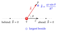
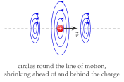
Compare Eq. (4.1.9) with Coulomb's field, $E = q R / (4 π ε_{0} R^{3})$ . Both fall off as $1/ R^{2}$ and both are proportional to the charge, but the electric field points along $R$ while the magnetic field is perpendicular to $R$ and to $v$ (Figure 4.1.4). Straight ahead of the charge, where $v ∥ R$ , there is no magnetic field at all. Exercise 4.1.3 puts numbers in and shows that for a charge moving at speed $v$ the ratio of the two fields is $B / E = v / c^{2}$ : magnetism is a small effect of motion, visible in a wire only because the wire is electrically neutral and the huge electric forces cancel.

The general form and the magnetic field H

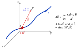
A current is a swarm of moving charges, so by superposition we add the contributions (4.1.9) of all of them. In a volume element $d v^{'}$ at the source point Q the moving charge is $ρ d v^{'}$ and $q v$ becomes $ρ v d v^{'} = J d v^{'}$ . Summing over the whole current distribution $V$ , Biot–Savart's law can be written in a general form as

Biot–Savart's law

B = \frac{μ _{0}}{4 π} \int_{V} J \times \frac{R}{R ^{3}} d v^{'} [T], (4.1.10)

with $R$ the vector from the source point Q (where $J$ is) to the field point P (where $B$ is wanted), $d v^{'} = d x^{'} d y^{'} d z^{'}$ , and the integral taken over the primed source coordinates. The magnetic field $H$ is defined as

H = \frac{B}{μ _{0}} = \frac{1}{4 π} \int_{V} J \times \frac{R}{R ^{3}} d v^{'} [A/m] . (4.1.11)

In the above equations $μ_{0}$ is the permeability of free space, and it is replaced with $μ$ in other media. This issue will be discussed later in this chapter. Notice that $H$ does not contain $μ_{0}$ at all: like $D$ in electrostatics, it is fixed by the sources and the geometry alone, and its unit, the ampere per metre, says so. This is why the problems of this section are mostly worked in terms of $H$ , with $B = μ_{0} H$ added at the end when a force or a flux is wanted.

For a thin wire and for a current sheet the volume element collapses, as explained in Section 4.1.2, and the law takes the forms used in the problems:

B H a_{R} = \frac{μ _{0}}{4 π} \int_{C} \frac{I d l ^{'} \times R}{R ^{3}} (wire), = \frac{1}{4 π} \int_{S} \frac{J _{S} \times a _{R}}{R ^{2}} d S^{'} (sheet), = \frac{R}{R} . (4.1.12)

Biot–Savart's law for a wire. The element I\,d\vec l' at the source point Q contributes at P a field d\vec B perpendicular to the plane of d\vec l' and \vec R, of magnitude \mu_0I\,dl'\sin\alpha/(4\pi R^2) with \alpha the angle between them. The total field is the vector sum of all elements. Problems 4.1.1 and 4.1.2 carry out this sum for a straight wire and for a circular loop. — **Figure 4.1.5.** Biot–Savart's law for a wire. The element $I d l^{'}$ at the source point Q contributes at P a field $d B$ perpendicular to the plane of $d l^{'}$ and $R$ , of magnitude $μ_{0} I d l^{'} sin α / (4 π R^{2})$ with $α$ the angle between them. The total field is the vector sum of all elements. Problems 4.1.1 and 4.1.2 carry out this sum for a straight wire and for a circular loop.

The probe sums $I d l^{'} \times R / R^{3}$ numerically over both wires. Switch between parallel and antiparallel currents to see superposition at work.

InteractiveLoading simulation…

In plain words

Every bit of current is a little source of magnetic field. Its field circles round it, falls off as $1/ R^{2}$ , and is strongest beside the element and zero in line with it. Add the little circles of all the bits and you have the field of the whole current.

Common mistake · The direction of R

Taking $R$ from the field point to the source. As in Coulomb's law, $R$ runs from the source point Q (the current element) to the field point P. With $R$ reversed, $B$ comes out with the wrong sign, and because $B$ enters the force through a vector product, the force is then reversed too. A second check is always available: the field of a straight current circles it in the sense of the right hand with the thumb along the current.

μ0 after the 2019 revision of the SI

Until 2019 the ampere was defined through the force between two parallel wires (Worked example 4.1.1), which made $μ_{0}$ exactly $4 π \times 1 0^{- 7}$ H/m. Since 20 May 2019 the ampere is fixed by the elementary charge, $e = 1.602176634 \times 1 0^{- 19}$ C, so $μ_{0}$ is now a measured quantity: $1.25663706212 (19) \times 1 0^{- 6}$ H/m (CODATA 2018), above $4 π \times 1 0^{- 7}$ H/m by $5.4 \times 1 0^{- 10}$ in relative terms. The value $4 π \times 1 0^{- 7}$ H/m stays exact enough for anything in this book.

Quick check

A short straight element $I d l^{'} = 2 A \times 1 mm a_{z}$ sits at the origin. What is $d B$ at the point $(0.1, 0, 0)$ m? And at $(0, 0, 0.1)$ m?

At $(0.1, 0, 0)$ : $R = 0.1 a_{x}$ , $a_{z} \times a_{x} = a_{y}$ , so $d B = 1 0^{- 7} \times 2 \times 1 0^{- 3} /0.01 = 2 \times 1 0^{- 8}$ T along $a_{y}$ , i.e. $20$ nT. At $(0, 0, 0.1)$ : $R ∥ d l^{'}$ , so $d B = 0$ .

4.1.3 Biot–Savart's law

The field of a moving point charge

The general form and the magnetic field H