Electromagnetic Fields and Waves: Notes, Solved Problems and Interactive Lab

In electrostatics the field could be written as the gradient of a scalar, $E = - \nabla V$ , which simplified both the theory and the calculations. The magnetic field cannot be written this way, because its lines close on themselves and the line integral of $B$ round a closed path is not zero. But it can be written as the curl of a vector. The derivation is short and uses one identity.

Rewriting Biot–Savart's law

Start from Biot–Savart's law (4.1.10),

B = \frac{μ _{0}}{4 π} \int_{V} J \times \frac{R}{R ^{3}} d v^{'} .

We make use of the gradient of $1/ R$ with respect to the field point P (Section 2.2 and the Coulomb potential of Section 3.3),

\nabla_{P} (\frac{1}{R}) = - \frac{R}{R ^{3}}, (4.1.13)

to write

B = \frac{μ _{0}}{4 π} \int_{V} J \times \nabla_{P} (- \frac{1}{R}) d v^{'} .

Now the vector $J = J (Q)$ depends on the source point only, not on P, so it is a constant as far as $\nabla_{P}$ is concerned. The product rule for the curl of a scalar times a vector (Section 2.2) gives

\nabla_{P} \times [\frac{J ( Q )}{R}] = \frac{1}{R} = 0 [\nabla_{P} \times J (Q)] - J (Q) \times \nabla_{P} (\frac{1}{R}),

and the first term vanishes because $J (Q)$ does not depend on P. Then we get

J \times \nabla_{P} (- \frac{1}{R}) = \nabla_{P} \times [\frac{J ( Q )}{R}], (4.1.14)

and the magnetic field becomes

B = \frac{μ _{0}}{4 π} \int_{V} \nabla_{P} \times [\frac{J}{R}] d v^{'} = \nabla \times {\frac{μ _{0}}{4 π} \int_{V} \frac{J}{R} d v^{'}},

where the curl, which acts on the field coordinates, has been taken outside the integral over the source coordinates. Here we define the vector potential.

The vector potential

A = \frac{μ _{0}}{4 π} \int_{V} \frac{J}{R} d v^{'} [Wb/m], with B = \nabla \times A . (4.1.15)

In plain words

Each current element contributes to $A$ a vector parallel to itself, weighted by $1/ R$ : $A$ "follows the current" and falls off like the scalar potential of a charge. The field $B$ is then the curl, the local rotation, of $A$ . Compare: a charge element contributes to $V$ a scalar weighted by $1/ R$ , and $E = - \nabla V$ .

The vector potential of a straight current. Every element I\,d\vec l' is along \vec a_z, so \vec A is along \vec a_z everywhere, parallel to the current and decreasing with the distance (Exercise 4.1.9 shows A_z\propto-\ln\rho). A vector field whose magnitude changes across its own direction has a curl: \nabla\times\vec A is the familiar circling field \vec B of Problem 4.1.1. — **Figure 4.1.6.** The vector potential of a straight current. Every element $I d l^{'}$ is along $a_{z}$ , so $A$ is along $a_{z}$ everywhere, parallel to the current and decreasing with the distance (Exercise 4.1.9 shows $A_{z} \propto - ln ρ$ ). A vector field whose magnitude changes across its own direction has a curl: $\nabla \times A$ is the familiar circling field $B$ of Problem 4.1.1.

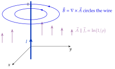
The unit of $A$ is the weber per metre, or equivalently the tesla metre and the volt second per metre. Like the scalar potential, $A$ is not unique: adding the gradient of any scalar function $ψ$ to $A$ does not change $B$ , because $\nabla \times \nabla ψ = 0$ (Section 2.2). For the infinitely long wire, $A$ itself is infinite but its differences are finite, exactly as for the potential of an infinite line charge (Exercise 4.1.9). Problem 4.1.8 computes $A$ for a flat ring of current and shows a pitfall: $A = 0$ at one point says nothing about $B$ there, because the curl needs $A$ in a neighbourhood of the point.

Quick check

In some region $A = \frac{1}{2} B_{0} (- y a_{x} + x a_{y})$ with $B_{0}$ constant. What is $B$ ?

$\nabla \times A = (\partial_{x} A_{y} - \partial_{y} A_{x}) a_{z} = \frac{1}{2} B_{0} (1 + 1) a_{z} = B_{0} a_{z}$ : a uniform field. The vector potential of a uniform field circles the $z$ -axis and grows with the distance, like the velocity of a rigidly rotating disk.

4.1.4 The vector potential

Rewriting Biot–Savart's law