4.1.7 Two fields every engineer should know

Two current distributions occur so often that their fields are worth knowing by heart. Both are derived in full in the problems at the end of the section, once with Biot–Savart's law and once, for the wire, with Ampère's law. Here we state the results and look at the pictures.

The infinitely long straight wire

A thin straight wire on the $z$-axis carrying $I$ along $+a_z$ produces at the normal distance $\rho$ (Problems 4.1.1 and 4.1.4)

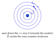
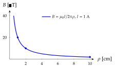
The lines of $H$ are circles centred on the wire (Figure 4.1.9a), in the sense of the right hand with the thumb along the current. The magnitude falls off as $1/\rho$, not $1/{\rho }^2$, for the same reason as the field of a line charge (Problem 3.2.1): moving away one sees more of the wire at once. With ${\mu }_0/2\pi =2\times 10^{-7}$ H/m the numbers are easy: $1$ A gives $20$ μT at $1$ cm and $2$ μT at $10$ cm (Figure 4.1.9b), and $10$ A matches the Earth's field of about $50$ μT at $4$ cm. The field only decays, it never vanishes: a single wire has no "outside".

Drag P: 1 A gives 20 μT at 1 cm, and $2\pi \rho H$ stays equal to $I$.

The circular loop

A circular loop of radius $b$ in the $xy$-plane carrying $I$ in the $+a_{\varphi }$ sense produces on its axis, at the height $h$ (Problem 4.1.2),

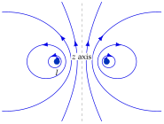
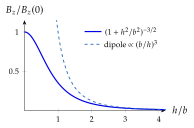
Off the axis there is no closed formula in elementary functions, but the field can be computed numerically, and Figure 4.1.10a shows the result: the lines go up through the loop, spread out, and come back down outside it to close round the wire. Close to the wire they are the circles of Figure 4.1.9a, bent round the loop. Far away the field is that of a magnetic dipole, falling as $1/h^3$ (Figure 4.1.10b), the counterpart of the electric dipole of Home exercise 3.1.4. A coil of $N$ turns multiplies everything by $N$, and stacking loops along the axis gives the solenoid of Home exercise 4.1.2.

Drag P off the axis: the numerical Biot–Savart sum matches the exact field computed with elliptic integrals.