Section 4.1 · Topic 9 of 11
4.1.9 Applications
The two laws of this section are the two halves of every magnetic device: Biot–Savart's law says what field a current makes, and the Lorentz force says what that field does to a moving charge or to another current. The four applications below use both. The first two follow the Lorentz force (a moving charge pushed sideways, a current-carrying wire pushed sideways), the third uses the field of the straight wire and Ampère's law read backwards, and the fourth uses the ring geometry of Problem 4.1.8. In the figures, means out of the page and into the page, is drawn blue, currents red and forces green.
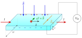
Send a current along a flat strip of thickness and width placed in a magnetic field normal to its face (Figure 4.1.13). E. H. Hall discovered in 1879 what happens. Each carrier, drifting along the strip with velocity , feels the Lorentz force sideways, across the width. The carriers are deflected towards one long edge, charge piles up there (and the opposite charge is left on the other edge), and a transverse electric field , the Hall field, builds up across the strip. The pile-up stops when the electric force on a carrier balances the magnetic one:
The current is (Section 4.1.2, with the carrier density and the cross-section), so , and the voltage between the two edges, the Hall voltage, is
Watch the edge charge build up until balances , switch between electrons and holes, then pick a semiconductor.
Three consequences make this simple effect one of the most used in electrical engineering.
- The sign of gives the type of the carriers, and gives their density . Electrons moving against end on the same edge as positive carriers moving with it (both and change sign in ), so the edge that goes positive tells which kind of carrier is present. This is how the carrier type and density of a semiconductor are measured.
- . In copper, with m, a strip of μm carrying A in T gives only μV (Worked example 4.1.2). Hall probes are therefore made of thin semiconductors (InSb, GaAs, Si) with to m, a million times fewer carriers and a million times more voltage: millivolts from a few milliamperes.
- at fixed . The element is a magnetometer, and when is produced by a current to be measured it becomes a contactless current sensor: the Hall element in the gap of the clamp meter of Application 4.1.3, the current sensors of motor drives and battery monitors. The same elements detect the rotor magnets of brushless DC motors and the teeth of a gear wheel, giving position and speed without contact.
A silicon Hall element with μm and m carrying mA in T gives mV, comfortably measured. Integrated Hall sensors add an amplifier on the same chip and output a voltage proportional to , or a switch that closes above a set field.
In a wire the moving charges are the carriers, and summing over a straight length gave the wire form of the Lorentz force, Eq. (4.1.5):
The current, not the carrier sign, fixes the direction. A m wire with A in T feels N. Put such a wire on a shaft and let it turn, and you have a motor.
The armature loop. Figure 4.1.14 shows the simplest DC motor: a rectangular loop of length and width on a shaft, in the field between the pole pieces N and S. The current runs opposite ways along the two long sides, so the two forces are equal and opposite: no net force on the loop, but a torque about the shaft. With the loop plane parallel to the lever arm of each force is and the torque is . In general, with the angle between and the normal of the loop, the lever arm is , and for a coil of turns
where is the area of one turn and is the magnetic moment of the coil.
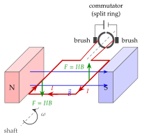
The commutator. As the loop turns, changes sign every half revolution and the torque would reverse: the loop would simply swing to the position and stop. The split ring and the fixed brushes reverse in the loop exactly when changes sign, so the torque is rectified to and always drives the same way. Its mean over a revolution is (Worked example 4.1.4). A real armature carries many coils spaced round the rotor, each commutated at its own moment, so the total torque stays close to instead of pulsating. A brushless motor replaces the commutator by electronic switches timed by Hall sensors (Application 4.1.1), but uses the same .
Run the coil with the commutator off in Free run, then switch it on and watch the torque keep one sign.
Worked example 4.1.4: a coil of turns, cm, cm, with A in a gap field of T feels N on each long side, gives N m and a mean torque of N m, and at rpm delivers about W, a hand-sized motor. The gap field of T is produced by permanent magnets or by field windings, and the iron of the rotor and poles concentrates it, a subject of the next section.
The field of the straight wire, Eq. (4.1.21), is the working formula of power engineering: with H/m. It is used in two opposite ways, to find the field of a known current and to find a current from its field.
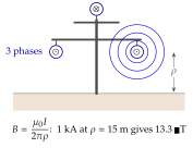
Under an overhead line. One conductor of a kV line, m above the ground, carrying kA, produces at the ground (Figure 4.1.15a and Worked example 4.1.3)
which is below the Earth's own static field of to μT at the surface, and about of the ICNIRP 2010 public reference level of μT at Hz. On a balanced three-phase line the three currents add to zero at every instant, so the three terms cancel and the resultant falls off as (Exercise 4.1.11 shows this for a go-and-return pair): a few microteslas under a real line. The single-conductor value is an upper bound.
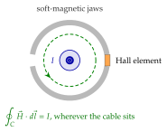
Reading a current from its field. Ampère's formula, , says that the circulation of round any closed loop equals the current through it. This is Problem 4.1.4 used backwards: on a circle of radius round a wire,
and more generally the circulation of round the loop gives the enclosed current whatever the shape of the loop and wherever the conductor sits inside it.
A clamp meter (Figure 4.1.15b) closes a soft-magnetic ring round one conductor. The iron gathers the flux of the wire's field, a winding on the ring reads an alternating current as a current transformer, and a Hall element in a sawn gap reads direct current too. Its signal depends only on the current inside the loop: the wire may sit anywhere in the jaw, and a neighbouring cable outside the jaw adds nothing, because its contributions to the circulation cancel round the loop (the mistake box of Section 4.1.5). Clamp the meter round a two-core cable carrying the go and the return current and it reads zero. In Worked example 4.1.3 a ring of mean radius cm round a A cable sees A/m, and A whatever the position of the cable.
A Rogowski coil (Figure 4.1.16) does the same without iron: a long flexible solenoid of turns per metre and cross-section is closed into a loop round the conductor. Each turn links the flux of the local field along the tangent of the loop, and the total flux linkage is
by Ampère's law, whatever the shape of the loop and the position of the conductor (Exercise 4.1.19). The coil contains no iron, so it never saturates: the same coil reads A and a kA fault current. So a current of kA in a busbar is measured without touching it, and the same law sets the clearance: kA at cm gives mT.
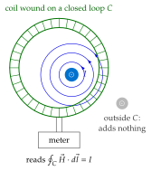
Worked example 4.1.3: kA at m gives μT, about a quarter of the Earth's field, and the field falls to μT only m away. A Rogowski coil with m and cm has μH and gives mV peak for a A rms, Hz current (Exercise 4.1.19).
A flat spiral wound from the radius to the radius carries its current in the direction on an annulus (Figure 4.1.17). Seen from more than a few turn-pitches away it is the sheet current of Problem 4.1.8: a surface current density on the ring , with for turns spread uniformly over the width .
The field at the centre is found by cutting the sheet into rings. The ring between and carries and, by Eq. (4.1.22) with , contributes at the centre. Hence, for turns spread uniformly from to ,
to be compared with for the same turns all placed at the radius .
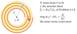
Wireless-charging pads (the Qi standard, to kHz), induction hobs (the bottom of the pan is the "receiver") and NFC antennas ( MHz) are all such coils. Because , the inner turns count most at the centre, while the outer turns add less there but extend the field further along the axis (Exercise 4.1.20): a charging pad wants a flat field over the receiver, so its turns are spread outward. At to kHz a pad coil runs with a few amperes and makes a few hundred microteslas, enough to transfer several watts across a few millimetres.
Twenty turns wound from to cm and carrying A: the sheet model gives kA/m at the centre, i.e. mT. Exercise 4.1.20 works the same coil wound from to cm: kA/m at the centre, falling to about half at the height .
Table 4.1.3. The applications of this section.
| Application | Physics used | Worked out in |
|---|---|---|
| Hall-effect sensor | on the carriers, | Worked example 4.1.2 |
| DC motor | , torque | Worked example 4.1.4 |
| Power lines and the clamp meter | , | Problems 4.1.1, 4.1.4, Worked example 4.1.3, Exercise 4.1.19 |
| Flat spiral coils | rings, | Problem 4.1.8, Exercise 4.1.20 |