Electromagnetic Fields and Waves: Notes, Solved Problems and Interactive Lab

Biot–Savart's law always works, but it means a vector integral for every problem: for the straight wire of Problem 4.1.1 it takes a page. Ampère's law in integral form, $\oint_{C} H \cdot d l = I_{enc}$ , does the same job in one line whenever the current distribution has enough symmetry, exactly as Gauss's law did for charges in Section 3.2. The exercise session of Lecture 9 is built on this idea, and its six problems are Problems 4.1.3–4.1.8 at the end of this section. Here we set out the method.

Symmetry first

Take the long straight wire on the $z$ -axis. Before writing any integral, ask what the symmetry allows (Figure 4.1.11):

A translation along $z$ and a rotation about $z$ leave the wire unchanged, so nothing can depend on $z$ or $ϕ$ : $H = H (ρ)$ .
A radial component $H_{ρ} (ρ)$ would give a non-zero flux of $B$ out of a coaxial cylinder, contradicting $\nabla \cdot B = 0$ (there is no magnetic charge on the axis to feed it): $H_{ρ} = 0$ .
A $z$ -component is excluded by Biot–Savart's law directly, since every element $I d z^{'} a_{z}$ gives $d B \propto a_{z} \times R$ , which has no $z$ -component. Equivalently, the mirror image of the wire in a plane containing it is the same wire with the same current, and the mirror image of $H_{z}$ would be $- H_{z}$ : $H_{z} = 0$ .

Only $H_{ϕ} (ρ)$ survives. On the circle $C$ of radius $ρ$ in a plane $z =$ const, traversed in the $+ a_{ϕ}$ sense, $H_{ϕ}$ is therefore constant and parallel to $d l = ρ d ϕ a_{ϕ}$ , so the circulation is simply $H_{ϕ} \times 2 π ρ$ . Such a path is called an Amperian path.

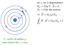
Symmetry first. For a long straight wire only H_\phi(\rho) survives, so on the circle C the field is constant and tangential and Ampère's law gives 2\pi\rho H_\phi=I_{\mathrm{enc}} at once (Problem 4.1.4). The same circle serves for a thick wire, a hollow wire and a coaxial cable: only the enclosed current changes. — **Figure 4.1.11.** Symmetry first. For a long straight wire only $H_{ϕ} (ρ)$ survives, so on the circle $C$ the field is constant and tangential and Ampère's law gives $2 π ρ H_{ϕ} = I_{enc}$ at once (Problem 4.1.4). The same circle serves for a thick wire, a hollow wire and a coaxial cable: only the enclosed current changes.

The symmetry rule for Ampère's law

Ampère's law gives the field directly whenever you can draw a closed path through the field point on which $H$ is either tangential with constant magnitude or perpendicular to the path. Then $\oint_{C} H \cdot d l = H \times (length of the tangential part) = I_{enc}$ , and $H$ follows by one division.

Three geometries have this property, and they are the magnetic counterparts of the three Gaussian surfaces of Table 3.2.1:

cylindrical symmetry (straight wires, tubes, coaxial cables): a coaxial circle, circulation $2 π ρ H_{ϕ}$ (Problems 4.1.4–4.1.7, Home exercises 4.1.5–4.1.6),
a long solenoid or a plane current sheet: a rectangle with one side in the field and the other where the field is zero or opposite, circulation $H ℓ$ or $2 H ℓ$ (Home exercise 4.1.7, Exercise 4.1.13), and
a toroid: a circle threading all the turns, circulation $2 π ρ H_{ϕ} = N I$ (Exercise 4.1.16).

Problems with only rotational symmetry about an axis, such as a spinning charged disk or a flat ring of current (Problems 4.1.3 and 4.1.8), do not have an Amperian path. For them the field on the axis is found by cutting the source into rings and adding the on-axis loop field (4.1.22), a one-dimensional integral instead of a one-line division.

The four-step recipe

Recipe · Ampère's law in four steps

Symmetry. Name the operations (translations, rotations, mirrors) that leave the current distribution unchanged and decide which component of $H$ survives, and on which coordinate it can depend.
Amperian path. Choose a closed path through the field point on which that component is constant (or on which parts of the path are perpendicular to $H$ ). If no such path exists, cut the source into rings and use the on-axis loop field instead.
Enclosed current. Compute the current through the surface spanned by the path, with the sign given by the right-hand rule: only the part of the current inside the path counts. Then $\oint_{C} H \cdot d l = I_{enc}$ gives $H$ .
Check the limits. Continuity of $H$ at every boundary without a surface current, the behaviour for $ρ \to 0$ and $ρ \to \infty$ , and the units (A/m).

**Figure 4.1.12.** The four-step recipe and how the six problems of the exercise session (Problems 4.1.3–4.1.8) fit it. Problems 4.1.4–4.1.7 have cylindrical symmetry and fall to one line of Ampère's law. Problems 4.1.3 and 4.1.8 have rotational symmetry about an axis and fall to a one-dimensional integral over rings.

Walk through the four steps: drag the circle across the hole, the metal and the air, and watch only the threaded current count.

InteractiveLoading simulation…

Problem	Symmetry and path	Enclosed current	Check
4.1.3	rotation about $z$ $\Rightarrow$ $B_{z}$ only, path: rings $d I = ρ_{S} ω ρ^{'} d ρ^{'}$	integrate the loop formula	$h = 0$ , $h ≫ b$
4.1.4	no $z$ , no $ϕ$ $\Rightarrow$ $H_{ϕ} (ρ)$ , path: circle $ρ = const$	$I$	matches Biot–Savart
4.1.5	as 4.1.4, path: same circle, in and out	$I ρ^{2} / b^{2}$ , then $I$	continuous at $ρ = b$
4.1.6	as 4.1.4, path: same circle, 3 regions	$0$ , $I (ρ^{2} - a^{2}) / (b^{2} - a^{2})$ , $I$	$a \to 0$ gives 4.1.5
4.1.7	$H$ given, then $J = \nabla \times H$ , then $ρ = b$	$400 π b$ both ways	continuous at $b$
4.1.8	rotation about $z$ , path: rings $d H_{z} = d I /2 ρ^{'}$	integrate $b \to 2 b$	sign of $sin (π ρ^{'} / b)$

Common mistake · A path on which H is not constant

Drawing a circle round a finite straight wire, or round a loop off its axis, and writing $\oint H \cdot d l = H \times 2 π ρ$ . Ampère's law still holds on such a path (the circulation is $I_{enc}$ ), but $H$ varies along it, so $H$ cannot be taken out of the integral and nothing can be extracted. Exercise 4.1.4 shows that the field of a finite segment depends on the angles under which its ends are seen, which no circle can know. Choose the path after the symmetry argument, never before.

Common mistake · Enclosed current means enclosed

Writing $I_{enc} = I$ for a circle drawn inside a thick wire. Only the current threading the circle counts: for a uniform current density it is $I ρ^{2} / b^{2}$ (Problem 4.1.5), for a hollow conductor $I (ρ^{2} - a^{2}) / (b^{2} - a^{2})$ (Problem 4.1.6), and for a non-uniform density it must be integrated (Home exercise 4.1.5). Conversely, a go-and-return pair encloses zero net current on any path round both wires, and yet $H$ is not zero there (Exercise 4.1.11).

Common mistake · The sign and the right hand

Traversing $C$ clockwise while counting the current positive along $+ z$ . The sense of $C$ and the positive direction of $I_{enc}$ are tied by the right hand: thumb along the current, fingers along $C$ . With the wrong pairing $H_{ϕ}$ comes out negative and the field circles the wrong way.

Where these six geometries turn up

Each problem of the exercise session is the textbook version of a geometry that engineers meet every day. Table 4.1.2 says where.

Table 4.1.2. Where the six geometries of Problems 4.1.3–4.1.8 turn up.

Problem	Geometry	Where it turns up
4.1.3	spinning charged disk	rotating machines, and the magnetic moment of a spinning charge (Rowland's experiment of 1876, the belt of a Van de Graaff generator)
4.1.4	straight wire	the $1/ ρ$ field round every cable, from which clamp meters read the current (Application 4.1.3)
4.1.5, 4.1.6	solid and hollow conductors	the field inside busbars and tubes, and a preview of the skin effect, which pushes the current of a high-frequency conductor into a thin shell
4.1.7	a given $H$	finding the current from the field, $J = \nabla \times H$ : Ampère's law read backwards
4.1.8	ring with a surface current	flat (pancake) coils: wireless-charging pads, induction hobs, NFC antennas (Application 4.1.4)

The one idea behind all six

Name the symmetry first. Problems 4.1.4–4.1.7 have cylindrical symmetry and fall to one line of Ampère's law. Problems 4.1.3 and 4.1.8 have rotational symmetry about an axis and fall to a one-dimensional integral over rings, using the on-axis loop field of Problem 4.1.2. In every case the symmetry decides which component of $H$ survives before any integral is written, and the check at the end (continuity, the limits $ρ \to 0$ and $ρ \to \infty$ , the units) catches most errors.

Quick check

Could Ampère's law be used to find the field at the centre of a square loop? And the field inside a long solenoid?

Not for the square: no closed path through the centre has a constant tangential $H$ (the field is found by Biot–Savart on the four sides, Home exercise 4.1.1). Yes for the solenoid: a rectangle with one side inside and one outside, Home exercise 4.1.7, gives $H = n I$ in one line.

4.1.8 Ampère's law at work

Symmetry first

The four-step recipe

Where these six geometries turn up